Supervised Machine Learning for Sample Classification in Drug Discovery: A 2025 Guide for Researchers
This article provides a comprehensive guide for researchers and drug development professionals on applying supervised machine learning for sample classification.
Supervised Machine Learning for Sample Classification in Drug Discovery: A 2025 Guide for Researchers
Abstract
This article provides a comprehensive guide for researchers and drug development professionals on applying supervised machine learning for sample classification. It covers foundational principles, key algorithms like Random Forests and SVMs, and their specific applications in biomedical contexts such as patient stratification, toxicity prediction, and disease diagnosis. The content addresses common challenges including data imbalance and overfitting, explores validation techniques and comparisons with self-supervised methods, and offers practical insights for implementing robust, interpretable models to accelerate drug discovery and development.
Understanding Supervised Learning: Core Concepts and Its Vital Role in Biomedical Sample Classification
What is Supervised Learning? Defining Labeled Data and the Learning Process
Supervised learning is a fundamental paradigm in machine learning where an algorithm learns to map input data to specific outputs based on example input-output pairs [1] [2]. This process involves training a statistical model using labeled data, meaning each piece of input data is provided with the correct output or answer [3] [4]. The primary goal is to create a model that can generalize from the training examples and accurately predict outputs for new, unseen data [1] [2]. In the context of sample classification research, such as classifying cell types or disease states, supervised learning provides a framework for building predictive models from known examples, enabling researchers to classify new, uncharacterized samples based on learned patterns [5] [6].
The "supervision" in this learning approach comes from the labeled datasets used to train models, which provide a ground truth that explicitly teaches the model to identify relationships between input features and output labels [1]. These labeled datasets consist of sample data points along with their correct outputs, allowing the algorithm to adjust its parameters until the model has been fitted appropriately to minimize prediction errors [1] [7]. For drug development professionals and researchers, supervised learning offers a methodical approach to transform experimental data into predictive models that can inform decision-making processes in areas such as patient stratification, drug response prediction, and diagnostic classification [5] [8].
Core Concepts and Definitions
Labeled Data
Labeled data represents the foundational element of supervised learning, consisting of raw data that has been assigned meaningful labels to provide context and enable model training [3]. In a supervised learning context, each data point in a labeled dataset contains both input features and a corresponding target label [7] [4]. The features are the descriptive attributes or measurements that characterize each example, while the label represents the "answer" or value that the model needs to predict [7]. For example, in a medical diagnosis scenario, the features might include patient vital signs, lab results, and demographic information, while the label would indicate the presence or absence of a specific condition [5].
Labeled data provides the "supervision" that guides the learning process by establishing a ground truth against which the model can compare its predictions and adjust its parameters accordingly [1]. This ground truth data is typically verified against real-world outcomes, often through human annotation or measurement, and serves as the ideal outputs for any given input data during training [1]. The quality, size, and diversity of labeled datasets significantly impact model performance, with larger and more diverse datasets generally leading to models that can better generalize to new data [7].
The Learning Process
The supervised learning process follows a systematic workflow that transforms labeled data into a predictive model:
Data Collection and Preparation: Gathering a representative dataset containing input features and corresponding target labels [4] [6]. This step may involve data cleaning, handling missing values, and transforming raw data into a suitable format for analysis [4].
Model Selection: Choosing an appropriate algorithm based on the problem type (classification or regression), data characteristics, and performance requirements [2] [6].
Training: Feeding the training data into the chosen algorithm, allowing the model to learn patterns and relationships between inputs and outputs [7] [4]. During this phase, the model iteratively adjusts its parameters to minimize the difference between its predictions and the actual labels [7].
Evaluation: Assessing model performance using a separate test dataset not seen during training [7] [5]. This step measures how well the model generalizes to new data.
Deployment and Inference: Using the trained model to make predictions on new, unlabeled examples in real-world applications [7] [5].
This structured approach enables researchers to develop models that can classify samples, predict continuous outcomes, or identify patterns in complex biological data [5] [6].
Types of Supervised Learning
Classification
Classification represents a fundamental category of supervised learning where the goal is to assign input data to predefined categories or classes [1] [5]. In classification tasks, the target labels are discrete values representing different classes or groups [4]. This approach is particularly relevant to sample classification research, where the objective is to categorize samples into distinct groups based on their features [5] [6].
Classification problems can be further divided based on the number of classes involved:
- Binary Classification: Involves distinguishing between exactly two classes, such as classifying medical samples as "diseased" or "healthy," or predicting whether a patient will respond to a particular treatment [1] [4].
- Multiclass Classification: Involves categorizing data into more than two classes, such as classifying cell types into multiple categories or identifying different stages of disease progression [4].
Classification algorithms learn decision boundaries that separate different classes in the feature space, enabling them to assign appropriate labels to new, unclassified samples [1] [5]. In biomedical research, classification models support various applications including disease diagnosis, cancer cell classification, and patient stratification [5].
Regression
Regression constitutes the second major category of supervised learning, focusing on predicting continuous numerical values rather than discrete categories [1] [5]. In regression tasks, the target variable represents a quantifiable measure that exists on a continuous scale [1] [8]. This approach is essential when the research objective involves estimating numerical values rather than assigning class labels.
Regression analysis models the relationship between input features and a continuous output variable, enabling prediction of numerical outcomes [1] [6]. In pharmaceutical and biomedical research, regression techniques facilitate various applications:
- Predicting patient survival times or disease progression rates [6]
- Estimating drug dosage responses or compound potency [5]
- Forecasting biomarker expression levels [6]
- Modeling the relationship between genetic variants and quantitative traits [5]
While both classification and regression utilize labeled training data, they address fundamentally different types of prediction problems—categorical versus continuous—requiring different algorithmic approaches and evaluation metrics [5] [6].
Supervised Learning Workflow: A Protocol for Researchers
Protocol: End-to-End Model Development
Objective: To provide a standardized protocol for developing supervised learning models for sample classification in research settings.
Pre-requisites: Labeled dataset with known input-output pairs, computational environment with machine learning capabilities.
Table 1: Data Preparation Protocol
| Step | Procedure | Considerations |
|---|---|---|
| Data Collection | Gather representative labeled data with input features and corresponding target labels. | Ensure data quality and relevance to research question [2]. |
| Feature Representation | Transform raw input data into descriptive features. | Feature selection critically impacts model accuracy [2]. |
| Data Splitting | Partition dataset into training (~70-80%) and testing (~20-30%) subsets. | Maintain class distribution balance across splits [5]. |
| Data Preprocessing | Handle missing values, normalize features, address class imbalance. | Preprocessing reduces noise and improves model stability [4] [6]. |
Table 2: Model Training and Evaluation Protocol
| Step | Procedure | Considerations |
|---|---|---|
| Algorithm Selection | Choose appropriate algorithm based on problem type and data characteristics. | Consider bias-variance tradeoff and model interpretability needs [2] [6]. |
| Model Training | Feed training data to algorithm to learn input-output relationships. | Monitor learning curves to detect overfitting/underfitting [7]. |
| Hyperparameter Tuning | Optimize model parameters using validation set or cross-validation. | Systematic tuning improves model performance [5]. |
| Model Evaluation | Assess performance on held-out test set using appropriate metrics. | Use metrics aligned with research objectives [7] [6]. |
| Model Interpretation | Analyze feature importance and decision boundaries. | Critical for scientific validation and insight generation [6]. |
Supervised Learning Workflow
Protocol: Model Validation and Selection
Objective: To establish rigorous validation procedures for selecting optimal supervised learning models.
Table 3: Model Validation Protocol
| Step | Procedure | Purpose |
|---|---|---|
| Cross-Validation | Partition training data into k folds; train on k-1 folds, validate on held-out fold. | Maximize use of limited data while reducing overfitting [1] [6]. |
| Performance Metrics | Calculate classification accuracy, precision, recall, F1-score, ROC-AUC, or regression metrics (MSE, R²). | Quantify model performance using multiple perspectives [4] [6]. |
| Statistical Testing | Perform significance tests to compare different models or against baseline. | Ensure performance differences are statistically significant [6]. |
| Error Analysis | Examine examples where model predictions are incorrect. | Identify systematic weaknesses and guide improvements [2]. |
Essential Algorithms for Sample Classification
Algorithm Selection Guide
Selecting appropriate algorithms is critical for successful sample classification research. Different algorithms offer varying strengths in terms of accuracy, interpretability, computational efficiency, and ability to handle different data types [6].
Table 4: Supervised Learning Algorithms for Classification
| Algorithm | Best Suited For | Advantages | Limitations | Research Applications |
|---|---|---|---|---|
| Logistic Regression [1] [5] | Binary classification problems with linear relationships | Highly interpretable, fast training, probabilistic outputs | Limited capacity for complex nonlinear patterns | Initial feasibility studies, biomarker identification |
| Support Vector Machines (SVM) [1] [5] | High-dimensional data, clear margin of separation | Effective in high dimensions, memory efficient | Performance depends on kernel choice | Gene expression analysis, medical diagnosis |
| Decision Trees [5] [6] | Complex nonlinear relationships, interpretable models | Intuitive visualization, handles mixed data types | Prone to overfitting, unstable to small variations | Clinical decision rules, patient stratification |
| Random Forests [1] [5] | Large datasets with complex interactions | Reduces overfitting, handles missing data, feature importance | Less interpretable than single trees | Drug response prediction, multi-omics integration |
| K-Nearest Neighbors (KNN) [1] [5] | Small to medium datasets with meaningful distance metrics | Simple implementation, no training phase | Computationally intensive for large datasets | Cell type classification, pattern recognition |
Advanced Ensemble Methods
Ensemble methods combine multiple models to improve predictive performance and robustness beyond what can be achieved with individual algorithms [1]. These approaches are particularly valuable in research settings where prediction accuracy is paramount and sufficient computational resources are available.
Random Forests: Construct multiple decision trees during training and output the mode of classes (classification) or mean prediction (regression) of the individual trees [1] [5]. This approach reduces overfitting compared to single decision trees and provides natural feature importance measures [5].
Gradient Boosting: Builds models sequentially where each new model corrects errors made by previous models [5]. This approach typically achieves high performance but requires careful tuning of hyperparameters and computational resources [5].
Ensemble methods are particularly effective for complex classification tasks in biomedical research, such as integrating multi-omics data for patient stratification or predicting treatment outcomes from heterogeneous clinical data sources [5].
Research Reagent Solutions
Table 5: Essential Resources for Supervised Learning Research
| Resource Category | Specific Tools/Solutions | Function in Research |
|---|---|---|
| Data Labeling Platforms | Crowdsourcing platforms, expert annotation tools [9] | Generate high-quality labeled datasets for model training |
| Machine Learning Libraries | Scikit-learn, TensorFlow, PyTorch, MATLAB Statistics and ML Toolbox [6] | Provide implementations of algorithms and utilities |
| Model Evaluation Frameworks | Cross-validation utilities, metric calculation libraries [6] | Standardized assessment of model performance |
| Hyperparameter Optimization | Grid search, random search, Bayesian optimization tools [5] | Systematic tuning of model parameters |
| Feature Selection Tools | Filter methods, wrapper methods, embedded methods [2] | Identify most relevant variables for prediction |
Evaluation and Interpretation
Performance Metrics
Rigorous evaluation is essential for validating supervised learning models in research contexts. The choice of evaluation metrics should align with the specific research objectives and the consequences of different types of prediction errors [6].
Table 6: Model Evaluation Metrics
| Metric | Formula | Interpretation | When to Use |
|---|---|---|---|
| Accuracy | (TP+TN)/(TP+TN+FP+FN) | Overall correctness of predictions | Balanced class distributions |
| Precision | TP/(TP+FP) | Ability to avoid false positives | When false positives are costly |
| Recall (Sensitivity) | TP/(TP+FN) | Ability to identify all positives | When false negatives are dangerous |
| F1-Score | 2×(Precision×Recall)/(Precision+Recall) | Harmonic mean of precision and recall | Balanced view of both false positives and negatives |
| ROC-AUC | Area under ROC curve | Overall performance across classification thresholds | Compare models regardless of threshold |
Addressing Common Challenges
Several challenges frequently arise in supervised learning projects for sample classification:
Overfitting: When a model learns patterns specific to the training data that do not generalize to new data [2] [5]. Mitigation strategies include collecting more training data, applying regularization techniques, simplifying the model, using ensemble methods, and employing cross-validation [2] [5].
Data Bias: Models may learn and amplify biases present in training data [5]. Address through balanced sampling, collecting representative data, and auditing model predictions across subgroups [5].
Class Imbalance: When some classes are underrepresented in the training data [6]. Mitigation approaches include resampling techniques, class weighting, and anomaly detection methods [6].
Curse of Dimensionality: High-dimensional data with many features can confuse learning algorithms [2]. Address through feature selection, dimensionality reduction techniques, and regularization [2].
Advanced Applications in Research
Biomedical Implementation Scenarios
Supervised learning enables numerous advanced applications in biomedical research and drug development:
Drug Discovery and Repurposing: Predicting drug-target interactions, classifying compounds by mechanism of action, and identifying novel therapeutic applications for existing drugs [5] [8].
Personalized Medicine: Developing classifiers that predict individual patient responses to specific treatments based on genetic, clinical, and lifestyle factors [5] [8].
Diagnostic and Prognostic Models: Creating systems that classify medical images, identify disease subtypes from molecular data, or predict disease progression and patient outcomes [5] [6].
Biomarker Discovery: Identifying molecular signatures or clinical features that robustly classify disease states or treatment responses [5] [6].
These applications demonstrate how supervised learning transforms complex biomedical data into actionable models that can accelerate research and improve healthcare decisions.
From Raw Data to Predictions
Future Directions and Emerging Trends
The field of supervised learning continues to evolve with several emerging trends particularly relevant to sample classification research:
Automated Machine Learning (AutoML): Systems that automate the process of algorithm selection, hyperparameter tuning, and feature engineering [4].
Explainable AI (XAI): Methods that enhance model interpretability through feature importance measures, attention mechanisms, and model-agnostic explanation techniques [6].
Integration with Domain Knowledge: Approaches that incorporate existing biological knowledge and constraints into machine learning models [4].
Federated Learning: Frameworks that enable model training across multiple institutions without sharing sensitive data [4].
These advancements are making supervised learning more accessible, interpretable, and applicable to challenging research problems while addressing important considerations around reproducibility and data privacy.
Supervised learning provides a methodological framework for building predictive models from labeled data, offering powerful approaches for sample classification across biomedical research domains. The structured workflow encompassing data preparation, model selection, training, validation, and interpretation enables researchers to transform complex data into actionable insights. As the field advances with improved algorithms, visualization tools, and interpretation methods, supervised learning continues to grow in its capacity to address challenging classification problems in drug development and biomedical science. By adhering to rigorous protocols and maintaining focus on biological relevance, researchers can leverage these approaches to advance scientific discovery and translational applications.
In sample classification research within biomedical and drug development, selecting the appropriate supervised learning approach is a critical first step in building predictive models from empirical data. Supervised learning algorithms learn to map input data (your sample features) to specific outputs based on example input-output pairs, forming the foundation for most predictive tasks in scientific research [2]. The nature of the question you are asking of your data fundamentally determines whether your problem is one of classification or regression—a distinction that dictates everything from algorithm choice to evaluation methodology [10] [11].
This guide provides a structured framework for researchers to correctly identify their problem type and implement the corresponding analytical protocols, ensuring that predictive models for sample analysis are both statistically sound and biologically meaningful.
Core Concepts: Classification and Regression
Regression: Predicting Continuous Outcomes
Regression analysis is used when the target variable—the outcome you wish to predict—is a continuous numerical value [10] [12]. It models the relationship between independent variables (features) and a continuous dependent variable (target) to make quantitative predictions [11].
- Objective: To predict a quantity—answering "how much?" or "how many?" [10].
- Example Research Questions:
- What is the predicted IC50 value of a compound based on its chemical descriptors?
- How will varying a formulation parameter affect drug dissolution rate?
- What is the relationship between gene expression levels and patient survival time?
Classification: Predicting Categorical Labels
Classification is used when the target variable is categorical or discrete, meaning it can take on a limited set of values representing different classes or groups [10] [12].
- Objective: To assign a category—answering "which type?" or "what class?" [10].
- Example Research Questions:
- Does this tissue sample indicate a malignant or benign tumor? [11]
- Based on its structural fingerprint, does this molecule belong to a class of kinase inhibitors?
- Will this patient respond to a specific therapy based on their biomarker profile?
The table below summarizes the fundamental differences between regression and classification tasks to guide initial task selection.
Table 1: Fundamental Differences Between Regression and Classification Tasks
| Feature | Regression | Classification |
|---|---|---|
| Output Type | Continuous numerical value (e.g., concentration, EC50, binding affinity) [12] | Categorical label (e.g., 'Toxic'/'Non-Toxic', 'Responder'/'Non-Responder') [12] |
| Primary Goal | Fit a line or curve that minimizes prediction error (e.g., least squares) [12] [11] | Learn a decision boundary that separates classes and minimizes misclassification [12] |
| Common Algorithms | Linear Regression, Polynomial Regression, Ridge/Lasso, SVR [10] | Logistic Regression, SVM, Decision Trees, Random Forest, k-NN [10] [1] |
| Model Output | A specific numerical value on a continuous scale. | A probability of class membership or a direct class label assignment [11]. |
| Primary Evaluation Metrics | Root Mean Squared Error (RMSE), Mean Absolute Error (MAE), R-squared [10] | Accuracy, Precision, Recall, F1-Score, AUC-ROC [10] [12] |
A Decision Framework for Researchers
Choosing the correct task requires a systematic examination of your research objective and data. The following protocol provides a step-by-step methodology.
Protocol: Task Selection and Model Setup
Objective: To provide a standardized procedure for determining the appropriate supervised learning task (classification or regression) and initiating model development.
Materials:
- Dataset with feature matrix (X) and target variable (y)
- Computational environment (e.g., Python with scikit-learn, R)
- Domain knowledge regarding the biological or chemical context
Procedure:
Define the Research Objective Formally:
- Phrase your goal as a specific question.
- Regression Trigger Words: "Predict the value of...", "Forecast the magnitude...", "Model the relationship between X and level of Y".
- Classification Trigger Words: "Identify whether...", "Categorize into group A or B...", "Diagnose the presence of...".
Analyze the Target Variable (Critical Step):
- Inspect the data type and nature of your target variable (y).
- Continuous Target: If the target is numerical and the intervals between values are meaningful (e.g., IC50 = 1.2 µM, 2.5 µM, 5.1 µM), proceed to regression [10].
- Categorical Target: If the target is a label, class, or status (e.g., "High", "Medium", "Low"; or "Active", "Inactive"), proceed to classification [10].
- Note: Ordinal categories (e.g., toxicity severity scores of 1, 2, 3) can sometimes be approached with either method, depending on the goal, but are often best handled by specialized ordinal classification techniques.
Select an Appropriate Algorithm:
- Based on the outcome of Step 2, select a suitable starting algorithm from Table 1.
- For Regression: Begin with Linear Regression for linear relationships or Random Forest Regression for complex, non-linear relationships.
- For Classification: Begin with Logistic Regression for binary outcomes or Random Forest Classification for multi-class problems and complex decision boundaries [10].
Define the Evaluation Metric a Priori:
- For Regression: Pre-specify an error metric like RMSE or MAE. The choice depends on whether you need to penalize large errors heavily (RMSE) or not (MAE) [12].
- For Classification: Pre-specify metrics based on the business/research cost of errors. For imbalanced datasets (e.g., rare event detection), prioritize Precision, Recall, and F1-Score over raw Accuracy [10].
Implement and Validate the Model:
- Split data into training, validation, and test sets.
- Train the model on the training set.
- Tune hyperparameters using the validation set.
- Report final performance only on the held-out test set to obtain an unbiased estimate of generalization error [2].
Application Notes and Experimental Protocols
Application Note 1: Predicting Compound Potency (Regression)
Research Context: In early drug discovery, predicting the continuous potency (e.g., IC50, Ki) of novel chemical compounds based on molecular descriptors saves significant synthetic and screening resources.
Protocol: Regression Analysis for IC50 Prediction
Data Preparation:
- Input Features (X): Calculate molecular descriptors (e.g., molecular weight, logP, polar surface area, number of rotatable bonds) or use fingerprints for a library of compounds.
- Target Variable (y): Collect experimentally determined pIC50 (-logIC50) values for a training set of compounds. The logarithmic transformation often improves model performance by normalizing the value distribution.
- Data Cleaning: Handle missing values (e.g., imputation or removal). Scale features to a similar range (e.g., StandardScaler in scikit-learn) as many algorithms are sensitive to feature magnitudes [2].
Model Training:
- Split the data (e.g., 70% training, 15% validation, 15% test).
- Train a Random Forest Regressor as a robust, non-linear starting model.
- Use the validation set to tune hyperparameters such as
n_estimators(number of trees) andmax_depth(tree depth) to prevent overfitting.
Model Evaluation:
- Predict pIC50 values for the test set compounds.
- Calculate RMSE and R-squared.
- Interpretation: An RMSE of 0.5 in pIC50 units implies the model's predictions are typically within ~0.5 log units of the true value. An R-squared of 0.7 indicates that 70% of the variance in pIC50 is explained by the model.
Application Note 2: Classifying Compound Mechanism of Action (Classification)
Research Context: Accurately categorizing compounds by their putative Mechanism of Action (MoA) enables target deconvolution and understanding of polypharmacology.
Protocol: Multi-Class Classification for MoA Categorization
Data Preparation:
- Input Features (X): Use high-dimensional data such as gene expression profiles from cell lines treated with compounds (e.g., L1000 data) or high-content imaging features.
- Target Variable (y): Assign categorical MoA labels (e.g., "HDAC inhibitor", "Kinase inhibitor", "DNA damager") based on prior knowledge. Ensure a sufficient number of examples per class.
- Data Preprocessing: Perform dimensionality reduction (e.g., PCA) or feature selection to mitigate the "curse of dimensionality" [2]. Standardize features.
Model Training:
- Implement a Support Vector Machine (SVM) classifier with a non-linear kernel (e.g., RBF) to handle complex class boundaries.
- Use the validation set to optimize the regularization parameter
Cand kernel parameters.
Model Evaluation:
- Predict MoA labels for the test set.
- Generate a confusion matrix to visualize per-class performance.
- Report Precision and Recall for each MoA class, as overall accuracy can be misleading if class distribution is imbalanced. The F1-Score provides a single balanced metric per class.
The Scientist's Toolkit: Essential Research Reagents & Materials
Table 2: Key Reagent Solutions for Supervised Modelling in Sample Research
| Item | Function & Application Notes |
|---|---|
| scikit-learn (Python) | A comprehensive open-source library providing robust implementations of both classification (e.g., LogisticRegression, SVC) and regression (e.g., LinearRegression, RandomForestRegressor) algorithms [10]. |
| Labeled Training Dataset | A curated set of sample data (e.g., compounds, tissue samples) where each instance is paired with a known, validated output (the label). This is the ground truth essential for model training [1] [2]. |
| Molecular Descriptors / Feature Vectors | Quantitative representations of samples (e.g., chemical structures, biomarker panels). These form the input feature matrix (X) for the model. Quality and relevance of features are paramount. |
| Data Standardization Tool (e.g., StandardScaler) | A preprocessing module used to transform features to have a mean of 0 and standard deviation of 1. This is critical for algorithms like SVMs and those reliant on gradient descent [2]. |
| Cross-Validation Module (e.g., GridSearchCV) | A utility for automated hyperparameter tuning and model validation. It helps in finding the optimal model parameters while providing a robust estimate of model performance without overfitting the test set. |
Workflow Visualization for a Research Project
The following diagram outlines the end-to-end logical workflow for a typical supervised learning project in a research setting, incorporating the decision point between classification and regression.
Within the framework of supervised modelling for sample classification research, the selection of an appropriate algorithm is paramount to the success of drug development and biomedical studies. This document provides detailed application notes and experimental protocols for four cornerstone classification algorithms: Logistic Regression, Support Vector Machines (SVM), Random Forest, and Neural Networks. Each method offers a distinct balance of interpretability, flexibility, and predictive power, making them suitable for various stages of the research pipeline, from initial exploratory data analysis to final predictive model deployment. The following sections synthesize their theoretical bases, performance characteristics, and practical implementation workflows to guide researchers and scientists in their application.
Algorithm Performance Comparison
The choice of algorithm is often dictated by the dataset size, nature of the classification problem, and the need for interpretability versus pure predictive accuracy. The following table summarizes key performance metrics and characteristics to guide algorithm selection.
Table 1: Comparative Analysis of Classification Algorithms for Research Applications
| Algorithm | Ideal Dataset Size | Key Strengths | Key Limitations | Interpretability | Sample Performance Metrics |
|---|---|---|---|---|---|
| Logistic Regression | Very small (<100 samples) to moderate [13] | Probabilistic outputs, high speed, low computational cost, resilience to overfitting with regularization [14] [13] | Assumes linear relationship between features and log-odds; struggles with complex, non-linear patterns [13] | High (Provides feature coefficients) [14] [13] | Accuracy: Up to 94.58%; AUC: 0.85 on complex image data [14] |
| Support Vector Machine (SVM) | Small to moderate [13] | Effective in high-dimensional spaces; handles non-linear data via kernel trick; strong theoretical foundations [15] [13] [16] | Computationally intensive for large datasets; sensitive to hyperparameter tuning; less interpretable [13] [16] | Moderate to Low (Decision boundary defined by support vectors) [13] | High accuracy reported in image classification (e.g., 95% for skin lesions) [17] |
| Random Forest | Moderate (500+ samples) to large [13] | Handles non-linearity; robust to outliers and missing data; provides feature importance scores [18] [13] [19] | Computationally expensive; "black box" model; can overfit on very small datasets [18] [13] [19] | Moderate (Via feature importance) [19] | Outperforms logistic regression in ~69% of 243 real-world datasets [14] |
| Neural Networks | Large [20] | High accuracy; automatically learns feature hierarchies; models highly complex, non-linear patterns [21] [20] | High computational cost; requires large amounts of data; highly complex and opaque [21] [20] | Low (Complex "black box") [21] | Superior performance on complex tasks like image and speech recognition [21] |
Detailed Algorithmic Workflows
Logistic Regression
Logistic regression is a linear model that predicts the probability of a sample belonging to a particular class. It transforms a linear combination of input features using a sigmoid function to output a value between 0 and 1 [14] [13].
Figure 1: Logistic regression workflow for sample classification.
Experimental Protocol: Binary Classification for Medical Imaging
- Objective: To classify medical images (e.g., X-rays) as showing signs of disease (1) or not (0).
- Data Preprocessing: Standardize pixel intensity values to have a mean of 0 and a standard deviation of 1. Split data into training, validation, and test sets (e.g., 70/15/15).
- Model Training: Use Maximum Likelihood Estimation (MLE), often implemented via Iteratively Reweighted Least Squares (IRLS), to find the optimal coefficients (β) that minimize the binary cross-entropy loss function [14] [20].
- Regularization: Apply L1 (Lasso) or L2 (Ridge) regularization to prevent overfitting, especially with high-dimensional data [13].
- Evaluation: Assess model performance on the held-out test set using Area Under the ROC Curve (AUC), accuracy, and F1-score [14].
Support Vector Machines (SVM)
SVMs classify data by finding the optimal hyperplane that maximizes the margin between classes in a high-dimensional space. The samples closest to the hyperplane are the "support vectors" that define the classifier [15] [16].
Figure 2: SVM finds the hyperplane that maximizes the margin between two classes.
Experimental Protocol: Protein Classification using SVM
- Objective: Classify protein sequences into functional families based on their features.
- Feature Extraction: Generate features from protein sequences (e.g., amino acid composition, physicochemical properties).
- Kernel Selection: For non-linearly separable data, use the kernel trick. The Radial Basis Function (RBF) kernel is a common default choice [17] [16].
- Hyperparameter Tuning: Use grid search with cross-validation to find the optimal values for:
- C (Regularization): Controls the trade-off between achieving a low training error and a low testing error.
- Gamma (RBF kernel): Defines how far the influence of a single training example reaches [17].
- Model Evaluation: Report precision, recall, and accuracy on an independent test set. The model's decision function can be used to plot an ROC curve.
Random Forest
Random Forest is an ensemble method that constructs a multitude of decision trees at training time. The final classification is the mode of the classes output by individual trees, which reduces overfitting and improves generalization [18] [19].
Figure 3: Random Forest uses multiple decorrelated trees and aggregates their results.
Experimental Protocol: Drug Sensitivity Prediction
- Objective: Predict patient sensitivity to a drug based on genomic and clinical features.
- Data Preparation: Handle missing values (Random Forest can work with missing data, but imputation may still be beneficial). Ensure categorical variables are encoded.
- Model Training:
- Feature Importance: After training, extract the Gini importance or mean decrease in impurity to identify the genomic markers most predictive of drug response [18].
- Evaluation: Use accuracy and AUC. Perform cross-validation to obtain robust estimates of model performance and to mitigate overfitting.
Neural Networks
Neural networks consist of interconnected layers of artificial neurons that learn hierarchical representations of data. They are particularly powerful for complex patterns in high-dimensional data like images or genetic sequences [21] [20].
Figure 4: A simple feedforward neural network with multiple hidden layers.
Experimental Protocol: Image-Based Cell Phenotype Classification using CNN
- Objective: Classify microscope images of cells into different phenotypic categories.
- Architecture Selection: Use a Convolutional Neural Network (CNN), which is designed for image data [21].
- Training with Backpropagation:
- Optimizer: Use Adaptive Moment Estimation (Adam) for efficient convergence [20].
- Loss Function: For multi-class classification, use Categorical Cross-Entropy [20].
- Activation Function: Use ReLU in hidden layers to mitigate vanishing gradients and Softmax in the output layer to obtain class probabilities [20].
- Regularization: Employ techniques like Dropout and early stopping to prevent overfitting.
- Evaluation: Use a confusion matrix and top-1 accuracy on a test set of images not seen during training.
The Scientist's Toolkit: Essential Research Reagents & Software
The following table lists key software and libraries required for implementing the described classification algorithms in a research environment.
Table 2: Key Research Reagents and Software Solutions for Algorithm Implementation
| Item Name | Function / Application | Example Use Case |
|---|---|---|
| scikit-learn | A comprehensive open-source machine learning library for Python. | Provides efficient and easy-to-use implementations for Logistic Regression, SVM, and Random Forest [18] [19]. |
| PyTorch / TensorFlow | Open-source libraries for deep learning and numerical computation. | Used for building and training complex Neural Networks, including CNNs and RNNs [21] [22]. |
R e1071 / kernlab |
R packages for statistics and machine learning. | Contain functions for fitting Support Vector Machines with various kernels [15] [16]. |
| Weka | A Java-based workbench for machine learning and data mining. | Offers a GUI and API for applying a collection of classification algorithms, including Random Forest, without programming [16]. |
| Imbalanced Learn (sklearn-contrib) | A Python package providing techniques for handling imbalanced datasets. | Used for oversampling (SMOTE) or undersampling when one class is underrepresented, a common issue in medical datasets [17]. |
Supervised learning (SL), a foundational machine learning paradigm, has transitioned from an experimental tool to a core component of modern pharmaceutical research and development [23]. This methodology employs algorithms to learn from labeled datasets, where each example is paired with a known outcome, enabling the model to discern complex patterns and make predictions on new, unseen data [24]. In the context of drug discovery, these labels can represent a vast array of critical information, including a compound's biological activity, binding affinity for a target, toxicity profile, or a patient's likely response to a therapy [25] [26]. The ability to predict such outcomes from molecular or clinical data is fundamentally reducing the reliance on serendipity and labor-intensive trial-and-error approaches that have long characterized the field.
The transformative impact of SL stems from its direct addressal of the pharmaceutical industry's most pressing challenges: escalating costs, lengthy timelines, and high attrition rates [25] [27]. Traditional drug discovery can require over a decade and investments exceeding $2.5 billion per approved drug, with nearly 90% of candidates failing during clinical trials [27]. By providing data-driven predictions, SL enhances decision-making, prioritizes the most promising candidates, and derisks the development process. Its application spans the entire drug discovery and development pipeline, compressing timelines that once took years into months and substantially lowering associated costs [28] [25]. As of 2024, SL was the dominant algorithmic type in the machine learning drug discovery market, holding a 40% revenue share, a testament to its widespread adoption and proven utility [29].
Core Supervised Learning Algorithms and Their Pharmaceutical Applications
The power of supervised learning is realized through a suite of algorithms, each with distinct strengths suited to specific tasks in the drug discovery workflow. These models are broadly categorized based on their prediction target: classification for categorical outcomes and regression for continuous values [24].
Table 1: Key Supervised Learning Algorithms in Drug Discovery
| Algorithm | Learning Type | Primary Drug Discovery Applications | Brief Rationale |
|---|---|---|---|
| Random Forests | Classification, Regression | Virtual screening, toxicity prediction, patient stratification [27] [30] [29] | Robust, handles high-dimensional data, reduces overfitting via ensemble learning [24] [30]. |
| Support Vector Machines (SVM) | Classification, Regression | Compound classification, bioactivity prediction, image analysis (e.g., histology) [27] [26] [30] | Effective in high-dimensional spaces, finds optimal separation boundaries between classes [27] [30]. |
| Neural Networks/Deep Learning | Classification, Regression | De novo molecular design, ADMET prediction, advanced image recognition [27] [26] [29] | Captures highly complex, non-linear relationships in large, intricate datasets [26]. |
| Logistic Regression | Classification | Binary outcome prediction (e.g., active/inactive, toxic/non-toxic) [27] [30] | Provides a simple, interpretable baseline model for probabilistic classification [24] [30]. |
| Gradient Boosting (XGBoost, etc.) | Classification, Regression | Quantitative Structure-Activity Relationship (QSAR) modeling, predictive toxicology [24] [23] | State-of-the-art performance on structured data; builds models sequentially to correct errors [24]. |
The selection of an algorithm depends on the specific problem, data type, and dataset size. For instance, Random Forest and Gradient Boosting are frequently top performers for structured data from chemical assays, while Deep Neural Networks excel in tasks involving raw, complex data like molecular structures or medical images [24] [26]. The trend is moving towards increasingly sophisticated models, with the deep learning segment projected to be the fastest-growing in the coming years due to its power in structure-based predictions and generative design [29].
Application Notes: Supervised Learning Across the Drug Discovery Pipeline
Target Identification and Validation
The initial stage of drug discovery involves pinpointing a biological target (e.g., a protein) implicated in a disease. SL models are trained on diverse multi-omics data (genomics, proteomics) and vast scientific literature to identify and prioritize novel targets [25] [23]. For example, algorithms can be trained on labeled data linking specific gene mutations to disease phenotypes, enabling them to predict the causal role of new genes. A notable application is the identification of NAMPT as a therapeutic target in neuroendocrine prostate cancer through a computational drug discovery pipeline [23]. By analyzing complex biological data, these models can uncover previously unknown therapeutic targets, expanding the universe of treatable diseases.
Compound Screening and Lead Optimization
Once a target is identified, the search for a molecule that can effectively and safely modulate it begins. This phase has been revolutionized by SL.
- Virtual Screening: SL models can rapidly predict the binding affinity and biological activity of millions of compounds from virtual libraries, a process far more efficient than traditional high-throughput screening [25] [26]. Companies like Atomwise use convolutional neural networks to predict molecular interactions, having identified two drug candidates for Ebola in less than a day [25].
- Lead Optimization: This critical stage involves refining a "hit" compound into a "lead" candidate with optimal drug-like properties. SL dominates here, accounting for nearly 30% of the ML in drug discovery market share in 2024 [29]. Models are trained on historical data to predict key parameters such as potency, selectivity, and ADMET properties (Absorption, Distribution, Metabolism, Excretion, Toxicity) [26] [29]. Exscientia reports using such models to design drug candidates with 70% faster cycle times and requiring 10-fold fewer synthesized compounds than industry norms [28].
Clinical Trial Design and Patient Stratification
Clinical trials represent one of the most costly and high-attrition phases of drug development. SL is introducing much-needed efficiency and precision [25] [23].
- Patient Recruitment and Stratification: SL models analyze Electronic Health Records (EHRs), genetic data, and clinical notes to identify eligible patients for trials, significantly accelerating enrollment [25]. More importantly, they can stratify patients into subgroups based on their predicted response to therapy, enabling more targeted and powerful trials. For instance, ML models have been developed to predict metastasis in early-stage lung cancer or cognitive progression in Parkinson's patients, which can be used to enrich trial populations [23].
- Trial Outcome Prediction: SL helps design more efficient trials by predicting potential outcomes. This includes forecasting placebo response in major depressive disorder trials and predicting the risk of adverse events, such as edema in patients treated with tepotinib [23]. These insights allow for better trial design and patient monitoring, increasing the probability of success.
Table 2: Quantitative Impact of Supervised Learning in Drug Discovery
| Application Area | Exemplary Achievement | Impact Metric |
|---|---|---|
| Discovery Speed | Insilico Medicine's idiopathic pulmonary fibrosis drug candidate [28] [25] | Target discovery to Phase I trials achieved in 18 months (versus ~5 years traditionally) [28]. |
| Compound Efficiency | Exscientia's AI-designed compounds [28] | 70% faster design cycles and 10x fewer compounds synthesized than industry standards [28]. |
| Virtual Screening | Atomwise's screening for Ebola [25] | Two drug candidates identified in less than a day [25]. |
| Market Impact | Lead Optimization Segment [29] | Held ~30% share of the ML in drug discovery market in 2024 [29]. |
Experimental Protocols
Protocol 1: Building a QSAR Model for Activity Prediction
This protocol details the use of supervised learning to create a Quantitative Structure-Activity Relationship (QSAR) model that predicts a compound's biological activity from its chemical structure.
1. Problem Formulation & Data Collection
- Objective: To classify compounds as "active" or "inactive" against a specific protein target.
- Data Source: Public repositories like ChEMBL provide large, labeled datasets of chemical structures and their associated bioactivity measurements (e.g., IC50, Ki) [26].
- Label Definition: Compounds with potency (e.g., IC50) stronger than a defined threshold (e.g., < 1 µM) are labeled "active" (1); weaker compounds are labeled "inactive" (0).
2. Data Preparation and Featurization
- Featurization: Convert chemical structures (e.g., SMILES strings) into numerical descriptors that the model can process. Common features include:
- Molecular descriptors: Molecular weight, logP, number of hydrogen bond donors/acceptors.
- Fingerprints: Binary vectors indicating the presence or absence of specific chemical substructures.
- Data Splitting: Randomly split the dataset into a training set (~70-80%) to train the model, a validation set (~10-15%) for tuning hyperparameters, and a hold-out test set (~10-15%) for the final unbiased evaluation [24].
3. Model Training and Validation
- Algorithm Selection: Start with a robust, baseline algorithm like Random Forest [24].
- Training: The model learns the relationship between the input features (molecular descriptors) and the output labels (active/inactive) on the training set.
- Hyperparameter Tuning: Use the validation set to optimize model parameters (e.g., the number of trees in the forest) via techniques like grid search or random search.
4. Model Evaluation
- Metrics: Evaluate the final model on the untouched test set using classification metrics [24]:
- Accuracy: Overall correctness.
- Precision: Proportion of true actives among all predicted actives.
- Recall (Sensitivity): Proportion of true actives correctly identified.
- F1-Score: Harmonic mean of precision and recall.
- Confusion Matrix: A table visualizing true vs. predicted labels to understand the nature of errors.
The workflow for this QSAR modeling protocol is standardized and can be visualized as follows:
Protocol 2: Predicting Patient-Specific Toxicity from EHR Data
This protocol uses SL to predict a patient's risk of a specific adverse drug reaction (e.g., cisplatin-induced acute kidney injury) using clinical data [23].
1. Problem Formulation & Data Extraction
- Objective: To predict a binary outcome: whether a patient will experience a specific toxicity (e.g., Acute Kidney Injury) within a defined timeframe after treatment initiation.
- Data Source: Electronic Health Records (EHRs). Extract structured data (lab values, vital signs, demographics, medications) and/or unstructured clinical notes [23].
- Label Definition: Patients who developed the toxicity according to clinical criteria (e.g., KDIGO guidelines for AKI) are labeled "1" (case), and matched controls who did not are labeled "0".
2. Data Preprocessing and Feature Engineering
- Handling Missing Data: Impute missing lab values (e.g., using mean/median) or exclude variables with excessive missingness.
- Feature Engineering: Create predictive features from raw data:
- Data Splitting: Split patient-level data into training, validation, and test sets, ensuring all records from a single patient reside in only one set to prevent data leakage.
3. Model Training with Interpretability
- Algorithm Selection: Use interpretable models like Logistic Regression or Gradient Boosting (XGBoost) coupled with SHAP analysis for explainability [23].
- Training: Train the model on the training set to find the relationship between clinical features and toxicity risk.
- Interpretability: Apply SHAP (SHapley Additive exPlanations) analysis to understand which features (e.g., baseline creatinine, age) most heavily influenced the model's prediction, fostering clinical trust [23].
4. Model Validation and Performance Assessment
- Metrics: Evaluate performance on the test set. Key metrics include AUC-ROC (Area Under the Receiver Operating Characteristic curve) to assess overall ranking capability, and Precision-Recall curves, which are informative for imbalanced datasets [24].
- Clinical Validation: The model's predictions should be reviewed by clinical experts to ensure they are medically plausible before deployment.
The process for developing this clinical prediction model is outlined below:
The Scientist's Toolkit: Essential Research Reagent Solutions
The effective application of supervised learning requires a suite of computational "reagents" and data resources.
Table 3: Essential Research Reagent Solutions for Supervised Learning
| Tool/Resource Name | Type | Primary Function in SL Drug Discovery |
|---|---|---|
| ChEMBL [26] | Public Database | A manually curated database of bioactive molecules with drug-like properties, providing the labeled data essential for training models on bioactivity and binding affinity. |
| AlphaFold Protein Structure Database [25] [26] | Public Database | Provides highly accurate protein structure predictions, which serve as critical input features for structure-based SL models in virtual screening and target validation. |
| Amazon Web Services (AWS) / Google Cloud [28] [23] | Cloud Computing Platform | Offers scalable computational power and storage for training complex SL models on large datasets, with cloud-based deployment holding a ~70% market share in 2024 [29]. |
| SHAP (SHapley Additive exPlanations) [23] | Software Library | Provides post-hoc interpretability for "black box" models like neural networks and random forests, explaining which features drove a prediction to build trust with scientists and regulators. |
| Scikit-learn [24] | Software Library | A core Python library providing robust, efficient, and easy-to-use implementations of a wide variety of SL algorithms, from logistic regression to random forests. |
| TensorFlow/PyTorch [26] | Software Library | Open-source libraries for building and training deep neural networks, enabling complex tasks like de novo molecular design and advanced image-based phenotyping. |
| Electronic Health Records (EHRs) [25] [23] | Data Resource | A source of real-world patient data that, when properly curated and labeled, is used to train SL models for clinical trial recruitment, outcome prediction, and toxicity risk forecasting. |
Challenges and Future Outlook
Despite its promise, the implementation of supervised learning in drug discovery is not without hurdles. A primary challenge is the requirement for large, high-quality labeled datasets, which can be expensive and time-consuming to generate, particularly in domains like preclinical toxicology where data is scarce [30]. Furthermore, the issue of model interpretability remains significant; complex models like deep neural networks often function as "black boxes," making it difficult for researchers to understand the rationale behind a prediction, which can hinder trust and adoption in a highly regulated environment [30] [23]. Data bias and the potential for models to make unreliable predictions when faced with out-of-distribution data also pose substantial risks that must be managed [23].
The future of SL in drug discovery is bright and evolving. Key trends include the rise of Explainable AI (XAI) to demystify model decisions and the integration of SL with other AI paradigms [30] [23]. For instance, semi-supervised learning techniques are being developed to make better use of the vast amounts of unlabeled data available, mitigating the data-scarcity problem [31]. There is also a growing emphasis on creating AI-augmented workflows, where SL models do not replace scientists but rather empower them as "centaur chemists," providing data-driven insights to guide human intuition and experimentation [28]. As these technologies mature and overcome existing challenges, supervised learning is poised to become an even more deeply embedded infrastructure, accelerating the delivery of novel therapeutics to patients.
Supervised learning is a cornerstone of machine learning (ML) in scientific research, where models learn from labeled datasets to perform classification or prediction tasks [24]. For sample classification research—a critical component in fields like drug development and biomedical sciences—this involves training algorithms to categorize data into predefined classes based on input features [30]. The process enables enhanced decision-making by learning patterns from known examples where the "right answer" is provided, then applying these patterns to new, unlabeled data [24] [32].
The complete workflow extends far beyond initial model training, encompassing a structured, iterative pathway from problem definition through to continuous monitoring in production environments. This end-to-end process is essential for developing reliable, accurate, and generalizable models that can withstand the challenges of real-world application [24] [33]. In domains like healthcare research, robust supervised learning models (SMLMs) offer the potential to support complex prediction and classification tasks with speed and precision, thereby augmenting researcher capabilities and informing strategic decisions [32].
A successful supervised learning project for sample classification follows a structured, iterative workflow comprising five core stages [24]. This pathway ensures the development of a reliable and impactful model, from initial problem scoping to operational deployment and maintenance.
- Stage 1: Import and Frame the Data → This initial phase focuses on defining the research problem and gathering corresponding data. It involves framing a specific, measurable question and identifying what labeled data is needed to answer it [24].
- Stage 2: Data Preparation → The collected data must be cleaned, encoded, and scaled. New features are engineered, and the data is split into training, validation, and test sets to prevent bias in subsequent evaluation [24] [32].
- Stage 3: Choose and Train the Model → An appropriate algorithm is selected based on the problem type (e.g., classification). It is trained on the prepared data, often starting with a simple baseline model before progressing to more complex architectures [24].
- Stage 4: Evaluate and Validate → The model's performance is assessed on unseen test data using relevant metrics. This determines if its predictions are accurate and generalizable, or if further refinement is needed [24] [32].
- Stage 5: Deploy and Monitor → The validated model is put into a real-world production environment. Its performance is continuously tracked to detect any degradation over time, triggering retraining if necessary [24] [33].
This workflow is not strictly linear; it often requires iterating on previous steps based on findings from later stages [24]. For instance, performance issues detected during monitoring (Stage 5) may necessitate additional data preparation (Stage 2) or model retraining (Stage 3).
Phase 1: Data Framing and Preparation
Data Acquisition and Feature Selection
The foundation of any robust supervised learning model is high-quality, relevant data. The initial step involves acquiring a labeled dataset where each sample is associated with a known class or outcome [32]. For sample classification in research, features (independent variables) must be predictive of the target label (dependent variable). Domain knowledge is critical here for identifying meaningful features and designing informative data collection tools [32].
Redundant or irrelevant features increase model complexity and can reduce generalizability. Techniques like statistical tests, feature importance scores from tree-based models, and clinical domain expertise can help select the most predictive features [32].
Data Cleansing and Preprocessing Protocols
Raw data is often unsuitable for immediate model training and requires rigorous preparation. Key steps in this protocol include:
- Handling Missing Data: Common approaches include deletion of records or features with excessive missingness, or imputation using the mean, median, mode, or more advanced methods like K-nearest neighbors or multiple imputation by chained equations (MICE) [32].
- Data Encoding: ML models require numerical inputs. Categorical features must be encoded using techniques like one-hot encoding or label encoding [32].
- Feature Scaling: Variables on different scales can bias certain algorithms. Scaling values to a comparable range (e.g., [0, 1] or [-1, 1]) through normalization or standardization is often necessary [32].
Data Splitting Strategy
Prepared data must be partitioned into distinct sets to properly train and evaluate a model. A common practice is to allocate a larger portion (e.g., 70-80%) to the training set and the remainder to the testing set [32]. The training set is used to teach the model parameters, while the held-out test set provides an unbiased estimate of its performance on unseen data.
Phase 2: Model Selection and Training
Algorithm Selection for Sample Classification
The choice of algorithm depends on the problem nature, data size, and desired model interpretability. For sample classification research, several core algorithms are commonly employed [24] [30].
Table 1: Core Classification Algorithms for Sample Classification Research
| Algorithm | Primary Purpose | Key Applications in Research | Considerations |
|---|---|---|---|
| Logistic Regression [24] [30] | Models probability of a binary outcome. | Baseline modeling, medical diagnosis [30]. | Simple, fast, highly interpretable. |
| Decision Trees & Random Forests [24] [30] | Makes classification via a series of rules. Random Forest combines many trees. | Credit scoring, customer churn prediction, robust performance on structured data [24] [30]. | Random Forest is robust and often a strong performer. |
| Gradient Boosting (XGBoost, LightGBM) [24] | Sequentially builds models to correct errors of previous ones. | State-of-the-art performance on structured data [24]. | Powerful, but can be more complex to tune. |
| Support Vector Machines (SVM) [30] | Finds optimal boundary to separate classes in high-dimensional space. | Text categorization, image recognition, bioinformatics [30]. | Effective in high-dimensional spaces. |
| Naive Bayes [30] | Probabilistic classifier based on Bayes' theorem. | Text classification, sentiment analysis, spam detection [30]. | Performs well despite its simplifying assumptions. |
| Neural Networks [30] [32] | Captures complex, non-linear patterns through interconnected layers. | Image and speech recognition, complex pattern recognition [30] [32]. | Requires large data, less interpretable ("black box"). |
Model Training and Hyperparameter Tuning Protocol
Training involves using an algorithm to learn the relationship between features and labels from the training dataset. The algorithm iteratively adjusts its internal parameters to minimize prediction error [32]. A critical step in this phase is hyperparameter tuning. Hyperparameters are configuration external to the model itself (e.g., the depth of a tree, the learning rate of a neural network) that must be set before training [32].
A standard protocol for optimization is Grid Search with Cross-Validation (CV):
- Define a Hyperparameter Grid: Specify a set of possible values for each hyperparameter you wish to tune.
- Perform K-Fold Cross-Validation: For each combination of hyperparameters in the grid, the training data is split into k folds (e.g., k=5 or 10). The model is trained on k-1 folds and validated on the remaining fold, repeated k times so each fold serves as the validation set once.
- Select Optimal Configuration: The hyperparameter combination that yields the best average performance across all k validation folds is selected.
- Final Training: The model is retrained on the entire training set using these optimal hyperparameters [32].
Phase 3: Model Evaluation and Validation
Performance Metrics for Classification
Evaluating a model requires metrics that accurately reflect its performance on unseen data (the test set). Relying on a single metric can be misleading; a suite of metrics provides a comprehensive view [24].
Table 2: Key Evaluation Metrics for Classification Models
| Metric | Definition | Interpretation & Use Case |
|---|---|---|
| Accuracy [24] | Proportion of total correct predictions (both positive and negative). | Best when classes are balanced. Misleading with class imbalance. |
| Precision [24] | Proportion of positive predictions that were actually correct. | Critical when the cost of false positives is high (e.g., in spam detection). |
| Recall (Sensitivity) [24] | Proportion of actual positive cases that were successfully identified. | Critical when the cost of false negatives is high (e.g., in disease screening). |
| F1-Score [24] | Harmonic mean of Precision and Recall. | Provides a single score that balances both concerns. |
| Confusion Matrix [24] | A table showing true vs. predicted labels (True Positives, False Positives, True Negatives, False Negatives). | Gives a detailed breakdown of where the model is making errors. |
| Area Under the Receiver Operating Characteristic Curve (AUC) [33] | Measures the model's ability to distinguish between classes across all classification thresholds. | A value of 1.0 indicates perfect separation, 0.5 indicates no discriminative power. |
Validation in Practice: A Clinical Case Study
The Vent.io model, developed to predict the need for mechanical ventilation in ICU patients, demonstrates rigorous validation. The model was first trained and tested internally on data from one health system. It was then prospectively deployed in a "silent mode" where it made predictions in a real clinical environment without directing care, allowing for real-world validation which showed an AUC of 0.908 [33].
To test generalizability, the model was also validated on the external MIMIC-IV dataset. Here, its performance dropped to an AUC of 0.73, highlighting a common challenge: model performance can deteriorate when applied to data from different sources or populations [33]. This triggered a model fine-tuning process per a pre-defined plan, which successfully improved the AUC to 0.873 on the external dataset [33].
Phase 4: Model Deployment and Monitoring
Deployment Strategies and the Predetermined Change Control Plan (PCCP)
Deployment is the process of integrating a trained and validated model into a real-world environment to make predictions on new data. This can be done as a batch process or, more commonly, via a real-time API [24]. In regulated fields like healthcare, a Predetermined Change Control Plan (PCCP) is a critical component of deployment. A PCCP is a proactive strategy that outlines planned modifications to a model, the protocol for implementing them, and how to assess their impact [33].
The PCCP for the Vent.io model systematically tracked the model's AUC in production. It pre-specified an AUC threshold of 0.85; performance dropping below this level would automatically trigger model fine-tuning. This provides a structured, regulatory-compliant framework for maintaining model performance and safety over time [33].
Continuous Model Monitoring Framework
Once deployed, models are susceptible to performance decay due to changes in the underlying data environment. Continuous monitoring is essential to detect these issues [34].
Table 3: Key Metrics and Challenges in Production Model Monitoring
| Aspect to Monitor | Description | Common Challenges |
|---|---|---|
| Model Quality (Accuracy, Precision, etc.) [34] | Track performance metrics on new, labeled data as it becomes available. | Lack of Ground Truth: Labels for new data are often delayed, making real-time quality assessment impossible. Proxy metrics must be used [34]. |
| Data Drift [34] | Change in the statistical properties of the model's input features over time. | Requires comparing the distribution of live data to a reference (training) distribution, which is computationally intensive [34]. |
| Concept Drift [34] | Change in the relationship between the input features and the target variable. | Can be gradual (e.g., evolving user preferences) or sudden (e.g., a global pandemic), making it difficult to detect and attribute [34]. |
| Data Quality [34] | Issues with the incoming data, such as missing values, incorrect data types, or values outside expected ranges. | Bugs in upstream data pipelines can silently corrupt the model's inputs, leading to unreliable outputs without obvious system failures [34]. |
Silent failures are a key challenge in ML monitoring. Unlike traditional software that may crash, an ML model with corrupted input data will still produce a prediction, albeit a potentially low-quality one, without raising an alarm [34]. Monitoring must therefore be designed to detect these non-obvious errors.
The Scientist's Toolkit: Research Reagent Solutions
This table details key software and methodological "reagents" essential for implementing the supervised learning workflow for sample classification.
Table 4: Essential Research Reagents for Supervised Sample Classification
| Tool / Reagent | Type / Category | Primary Function in the Workflow |
|---|---|---|
| scikit-learn [24] | Python Library | Provides a unified interface for a wide array of ML algorithms (classification, regression, clustering) and essential utilities for model evaluation (metrics, train-test splits) and preprocessing (scalers, encoders). |
| XGBoost / LightGBM [24] | Algorithm Library | Offers high-performance, scalable implementations of gradient boosting frameworks, which are often top performers in classification tasks on structured data. |
| TensorFlow/PyTorch [33] [32] | Deep Learning Framework | Provides the foundation for building and training complex neural network models, from simple feedforward networks to advanced architectures for image or text data. |
| Evidently AI [34] | ML Monitoring Library | An open-source Python library specifically designed to calculate and track data and model quality metrics, detect drift, and visualize performance in production environments. |
| Pandas & NumPy [24] | Python Library | The fundamental packages for data manipulation and numerical computation. Used for loading, cleaning, transforming, and exploring datasets at all stages of the workflow. |
| Cross-Validation [32] | Methodology | A resampling procedure used to robustly assess model generalizability and tune hyperparameters when data is limited, by maximizing the use of available data for both training and validation. |
| Predetermined Change Control Plan (PCCP) [33] | Regulatory & Process Framework | A formal plan for managing post-deployment model changes, required for software as a medical device (SaMD) and critical for maintaining compliance and performance in regulated research. |
Integrated View: Connecting Workflow Phases
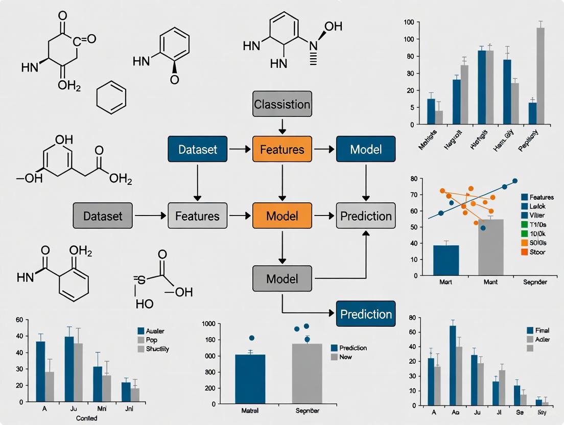
The following diagram synthesizes the core components of the supervised learning workflow, highlighting the critical processes, outputs, and feedback loops that connect data preparation to sustained performance in production.
This integrated view illustrates that model deployment is not an endpoint. The Monitoring System continuously validates the Deployed Model's Predictions, creating essential feedback loops. Alerts on data quality can trace back to the source Raw Data, while performance decay below a threshold, as governed by a PCCP, triggers model retraining. This closed-loop system is vital for maintaining a reliable and effective sample classification model in a dynamic research or clinical environment [24] [33] [34].
From Theory to Practice: Implementing Classification Models in Drug Development Pipelines
In the field of sample classification research, particularly within biological sciences and drug development, the selection of an appropriate supervised machine learning algorithm is a critical determinant of experimental success. This process must carefully balance model performance with interpretability, a consideration of paramount importance when research outcomes inform high-stakes decisions in areas like diagnostic marker identification or patient stratification. The core challenge for scientists lies in aligning the algorithmic choice with the specific characteristics of their dataset and the overarching goals of their classification task [35].
This guide provides a structured framework for this selection process, focusing on the interplay between data size, problem complexity, and analytical task. It moves beyond a theoretical discussion to offer application notes and detailed experimental protocols, providing a practical toolkit for researchers to systematically develop, evaluate, and deploy robust classification models. The principles outlined are universally applicable, yet are framed within the context of supervised modelling for sample classification, ensuring direct relevance to scientific research.
Core Principles of Algorithm Selection
Selecting a classification algorithm is not a one-size-fits-all process; it is a strategic decision based on a clear understanding of both the data and the project's objectives. The following principles provide a foundation for a reasoned and effective selection strategy.
Understand the Problem and Data Structure: The first step is to precisely define the classification problem, including the number of classes and the nature of the input features. A thorough exploratory data analysis is essential to understand data distribution, the presence of missing values, and potential outliers [24]. This phase should also characterize the dataset's scale, as this directly influences which algorithms are computationally feasible [36].
Evaluate the Need for Interpretability: In scientific research, the ability to interpret a model's predictions is often as important as its accuracy. For instance, understanding which genes or proteins a model uses for classification can yield novel biological insights. Linear models and decision trees offer high interpretability, whereas complex ensemble methods or neural networks are often "black boxes," though techniques like feature importance analysis can provide some post-hoc explanation [37] [35].
Prioritize Scalability and Computational Efficiency: The resource consumption of an algorithm—in terms of time and memory—must be considered, especially with large-scale omics data. Algorithmic complexity theory provides a framework for predicting how resource requirements grow with input size [36]. An algorithm that is efficient on a small, pilot dataset may become prohibitively slow or memory-intensive when applied to a full dataset, a common pitfall known as confusing "small-n performance with scalability" [36].
Adopt an Iterative Approach to Model Selection: Algorithm selection is rarely linear. It is best practice to start with a simple, interpretable model as a baseline (e.g., Logistic Regression) [24] [38]. The performance of this baseline can then be used to benchmark more complex models. This iterative process involves training multiple candidates, evaluating them rigorously using hold-out validation sets, and fine-tuning the most promising ones [24] [35].
A Structured Selection Framework
To operationalize the core principles, researchers can use the following decision framework, which matches algorithm families to common data and problem scenarios in sample classification. The subsequent table provides a quantitative summary for easy comparison.
Algorithm Selection Guide
| Algorithm Family | Typical Data Size | Handled Complexity | Primary Classification Task | Key Strengths | Key Weaknesses |
|---|---|---|---|---|---|
| Logistic Regression [38] | Small to Large | Linear | Binary, Multinomial | Highly interpretable, efficient, stable baseline [35] | Limited to linear decision boundaries |
| Decision Trees [39] | Small to Medium | Non-linear | Binary, Multinomial | Intuitive, handles mixed data, no strict scaling need [38] | Prone to overfitting, high variance |
| Random Forest [24] | Medium to Large | High, Non-linear | Binary, Multinomial | Robust, handles non-linearity, reduces overfitting [39] | Less interpretable, memory-intensive |
| Gradient Boosting (XGBoost, etc.) [24] | Medium to Large | High, Non-linear | Binary, Multinomial | State-of-the-art accuracy on structured data [24] | Requires careful tuning, computationally heavy |
| Support Vector Machine (SVM) [38] | Small to Medium | High, Non-linear (with kernel) | Binary | Effective in high-dimensional spaces (e.g., genomics) [38] | Poor scalability, slow on very large datasets |
| Naive Bayes [38] | Small to Large | Linear | Binary, Multinomial | Very fast, works well with high-dimensional data | Relies on strong feature independence assumption |
| K-Nearest Neighbor (KNN) [38] | Small | Instance-based | Binary, Multinomial | Simple, no training phase, naturally handles multi-class | Slow prediction, sensitive to irrelevant features |
| Neural Networks [40] [35] | Very Large | Very High, Non-linear | Binary, Multinomial | Superior for complex patterns (e.g., imaging) [40] | "Black box," needs massive data, computationally expensive [35] |
The workflow for navigating this framework begins with assessing the dataset size. For small to medium-sized datasets, a wide range of algorithms from Logistic Regression to SVMs are suitable. For very large datasets, efficient algorithms like Logistic Regression, Naive Bayes, or tree-based ensembles are preferable, with Neural Networks becoming a viable option only if data is truly massive and computational resources are available [36] [35].
Next, the complexity of the underlying problem must be considered. If the relationship between features and the class label is presumed to be simple and linear, Logistic Regression is an excellent starting point. For capturing complex, non-linear interactions, Decision Trees, Random Forests, Gradient Boosting, or Neural Networks are necessary [38] [35].
Finally, the need for interpretability is weighed against the desire for predictive power. In a regulatory context or for generating biological hypotheses, an interpretable model like a Decision Tree or Logistic Regression may be mandated. If the sole goal is maximum predictive accuracy for a well-defined task and the model will be used as a black-box tool, then Gradient Boosting or a Neural Network may be the optimal choice [37].
Algorithm Selection Workflow
Experimental Protocols for Model Evaluation
A rigorous, standardized protocol for training and evaluating models is fundamental for making unbiased comparisons between different algorithms. The following section outlines a core workflow and detailed methodology for this critical phase.
Standard Model Training and Evaluation Workflow
Protocol 1: Data Preprocessing and Partitioning
Objective: To transform raw data into a clean, structured format and partition it into training, validation, and test sets to enable unbiased model evaluation.
Methodology:
- Data Cleaning: Address missing values through removal or imputation (e.g., using mean, median, or k-nearest neighbors). Identify and manage outliers that could skew model training [24].
- Feature Scaling: Standardize or normalize numerical features to a common scale. This is critical for algorithms like SVMs and Logistic Regression that are sensitive to the magnitude of features [24].
- Data Splitting: Randomly split the dataset into three subsets:
- Training Set (~70%): Used to train the model.
- Validation Set (~15%): Used for hyperparameter tuning and model selection during development.
- Test Set (~15%): Held back entirely until the final model is chosen, providing an unbiased estimate of its performance on new data [24].
Protocol 2: Model Training and Hyperparameter Tuning
Objective: To train multiple candidate algorithms and optimize their hyperparameters using the training and validation sets.
Methodology:
- Baseline Model Training: Begin by training a simple baseline model, such as Logistic Regression, to establish a performance benchmark [24].
- Candidate Model Training: Train a diverse set of other algorithms (e.g., Random Forest, SVM, Gradient Boosting) on the training set.
- Hyperparameter Tuning: For each candidate model, perform a grid search or random search on the validation set to find the optimal hyperparameters (e.g., learning rate for boosting,
Cparameter for SVM, tree depth for Random Forest). Cross-validation within the training set can be used for a more robust tune [35].
Protocol 3: Performance Evaluation and Model Selection
Objective: To objectively compare the performance of tuned candidate models and select the best-performing one for final reporting.
Methodology:
- Validation Set Evaluation: Evaluate all tuned candidate models on the validation set to shortlist the top performers.
- Final Evaluation on Test Set: Take the shortlisted models (typically 1-3) and evaluate them only once on the held-out test set. This step provides an unbiased assessment of how the model will generalize to unseen data [24].
- Metric Selection:
- Model Interpretation: Analyze the final model to glean scientific insights. For tree-based models, examine feature importance. For linear models, review the coefficients [37].
The Scientist's Toolkit: Essential Research Reagents and Computational Solutions
In computational research, software libraries and hardware resources serve the same foundational role as laboratory reagents and equipment. The following table details key components of the modern data scientist's toolkit for sample classification.
| Tool Name / Solution | Category / Type | Function in Workflow | Example Use-Case in Classification |
|---|---|---|---|
| scikit-learn [24] [39] | Software Library | Provides unified API for data preprocessing, model training, and evaluation. | Implementing Logistic Regression, SVMs, Random Forests with few lines of code. |
| XGBoost / LightGBM [24] | Software Library | Highly optimized implementations of gradient boosting algorithms. | Achieving state-of-the-art accuracy on tabular genomic or proteomic data. |
| PyTorch / TensorFlow [40] | Software Library | Frameworks for building and training complex neural network models. | Developing custom deep learning models for image-based histopathology classification. |
| Pandas & NumPy [24] | Software Library | Core utilities for data manipulation, cleaning, and numerical computation. | Loading, cleaning, and transforming sample dataframes before model training. |
| High-RAM Computing Node | Hardware | Provides memory for holding and processing large datasets (e.g., full transcriptomes). | Training Random Forest models on large feature sets without memory overflow. |
| GPU (e.g., NVIDIA) [40] | Hardware | Accelerates compute-intensive matrix operations in deep learning and large-scale boosting. | Drastically reducing training time for neural networks and tree ensembles on big data. |
| Matplotlib / Seaborn [24] | Software Library | Generates static, interactive, and publication-quality visualizations for results. | Plotting ROC curves, confusion matrices, and feature importance graphs. |
Selecting the optimal machine learning algorithm for sample classification is a deliberate, multi-stage process that integrates data characteristics, computational constraints, and research objectives. There is no universal best algorithm; the most effective model is the one that most effectively balances performance, interpretability, and efficiency for a specific scientific question. By adhering to the structured framework and rigorous experimental protocols outlined in this guide, researchers and drug development professionals can make informed, defensible choices, thereby enhancing the reliability and impact of their computational research.
In sample classification research, the ability to accurately categorize data is foundational to generating reliable scientific insights. Supervised learning provides a powerful framework for this task, wherein an algorithm learns from a labeled dataset to make predictions on new, unseen data [1]. This process involves training a model to discern the underlying patterns and relationships between input features (the data you have) and target labels (the answers you want) [4]. For researchers and drug development professionals, building a robust classifier is not merely an algorithmic exercise but a critical step in transforming raw data into actionable knowledge, enabling applications from high-content screening analysis to patient stratification.
This protocol outlines a complete, step-by-step methodology for constructing a classifier, framed within the broader context of supervised modelling for research. It details the end-to-end workflow, from initial data preparation to final model deployment and monitoring [24]. The guide is designed to be practically actionable, providing detailed experimental procedures, structured data presentations, and clear visualizations to ensure that scientists can implement these methods effectively in their own work.
The Supervised Learning Workflow: A Five-Stage Process
A successful data science project follows a structured, iterative workflow to ensure a reliable and impactful result. While a project can be broken down into many micro-steps, it can be viewed as five main stages [24]:
- Import and Frame the Data: This initial stage is about defining the problem and gathering the necessary data. It involves framing a specific, measurable question, identifying what data is needed to answer it, and ensuring it is accessible and clean.
- Data Preparation: Before building a model, the data must be prepared. This is where you clean, encode, and scale your data, creating new features that will help the model learn more effectively. You will also carefully split the data into training, validation, and test sets to prevent bias in your evaluation.
- Choose the Model: With your data ready, you select and train a model. It’s often best to start with a simple model (a “baseline”) to ensure your more complex models are actually providing a benefit. You then train and tune your chosen model to optimize its performance.
- Evaluate: This stage is about assessing your model’s performance on the test data it has never seen before. You evaluate its accuracy using the right metrics and examine where it made errors to understand its limitations.
- Deploy and Monitor: The final stage is putting your model into the real world. You can deploy it as a batch job or an API. The work doesn’t stop here, though; it’s critical to continuously monitor the model’s performance for any “drift” in the data, ensuring it remains accurate over time and is still solving the problem it was designed for.
The following workflow diagram visualizes this iterative process:
Phase 1: Data Preparation and Curation
The lifeblood of any supervised learning model is high-quality, labeled data. The steps taken to prepare this data are critical to the ultimate performance and reliability of the classifier.
Data Collection and Labeling
The initial step involves gathering a dataset where each data point is associated with the correct output or answer; this is known as ground truth data [1]. For a spam email classifier, this would be a corpus of emails where each one is explicitly labeled as "spam" or "not spam" [24]. The quality and representativeness of this dataset are paramount, as the model will learn all its patterns from this information.
Data Preprocessing and Feature Engineering
Raw data is rarely suitable for immediate model training. It must be cleaned and transformed through a process often referred to as data curation [4]. This involves:
- Handling Missing Values: Addressing gaps in the data through techniques like imputation or removal.
- Removing Outliers or Inconsistencies: Identifying and mitigating data points that deviate significantly from the norm and could skew the model's learning.
- Feature Engineering: Creating new, more informative features from the raw data to help the model learn more effectively [24]. This can involve techniques like feature scaling (normalization or standardization) to ensure all features contribute equally to the model, and encoding categorical variables into a numerical format.
Data Splitting
Once the dataset is curated, it is essential to split it into subsets to properly train and evaluate the model [4]. A common practice is to split the data into:
- Training Set: The largest portion of the data (e.g., 70-80%) used to train the model and adjust its internal parameters.
- Validation Set: A smaller set (e.g., 10-15%) used to tune the model's hyperparameters and select the best performing model during training.
- Test Set: A hold-out set (e.g., 10-15%) used only once, at the very end, to provide an unbiased evaluation of the final model's performance on unseen data.
Table 1: Standard Data Splitting Protocol for Classifier Development
| Subset | Primary Function | Typical Proportion | Used for Final Performance Reporting? |
|---|---|---|---|
| Training Set | Model training and parameter adjustment | 70-80% | No |
| Validation Set | Hyperparameter tuning and model selection | 10-15% | No |
| Test Set | Unbiased final evaluation | 10-15% | Yes |
Phase 2: Model Selection and Training
With a prepared dataset, the next step is to select an appropriate algorithm and train it.
Types of Classification Algorithms
The choice of algorithm depends on the nature of the problem. Classification tasks can be binary (e.g., spam vs. not spam), multiclass (e.g., identifying different types of cells), or multi-label (where a single sample can belong to multiple categories simultaneously) [41]. Common algorithms include:
- Logistic Regression: A simple, fast, and interpretable model that provides a good baseline for classification problems [24].
- Decision Trees & Random Forests: Tree-based models that are intuitive and robust. Random Forest, an ensemble method, combines many decision trees to reduce overfitting and is often a strong performer [24] [1].
- Gradient Boosting (XGBoost, LightGBM): Powerful, state-of-the-art ensemble algorithms that build models sequentially, with each new model correcting the errors of the previous one. They are highly effective on structured data [24].
- Support Vector Machines (SVM): Effective for both classification and regression, SVMs plot a hyperplane to maximize the distance between different classes of data points [1].
- Naive Bayes: A classification algorithm based on Bayes' theorem, particularly useful for text classification and spam identification [1].
Table 2: Common Classification Algorithms and Their Characteristics
| Algorithm | Best Suited For | Key Advantages | Potential Limitations |
|---|---|---|---|
| Logistic Regression | Binary classification, linear problems | Simple, fast, interpretable, good baseline | Assumes linear relationship |
| Random Forest | Complex, non-linear problems, tabular data | High accuracy, robust to overfitting, handles mixed data types | Less interpretable, can be computationally heavy |
| Gradient Boosting | Complex problems where high performance is critical | Often state-of-the-art accuracy, flexible | Prone to overfitting without careful tuning, computationally intensive |
| Support Vector Machine (SVM) | High-dimensional data, complex non-linear boundaries | Effective in high dimensions, powerful with kernel tricks | Memory intensive, less effective on noisy data |
| Naive Bayes | Text classification, spam filtering | Fast, simple, works well with high-dimensional data | Relies on strong feature independence assumption |
The Training Process and Optimization
Training is the process where the model's algorithm processes the training dataset to explore potential correlations between inputs and outputs [1]. The model's optimization algorithm, such as Stochastic Gradient Descent (SGD), assesses accuracy through a loss function—an equation that measures the discrepancy between the model's predictions and the actual values [1]. Throughout training, the algorithm iteratively updates the model's parameters to minimize this loss, effectively "teaching" the model the correct relationships in the data. The following diagram illustrates the core training loop:
Phase 3: Model Evaluation and Validation
After training, the model must be rigorously evaluated to understand its real-world performance and limitations.
Key Evaluation Metrics for Classification
Choosing the right metric is crucial to avoid a false sense of security about your model's performance [24]. The most straightforward metric, accuracy, can be misleading if your classes are imbalanced. A more nuanced view comes from metrics derived from the confusion matrix, which provides a detailed breakdown of correct and incorrect predictions for each class [24].
- Accuracy: The percentage of correct predictions overall. (Can be misleading with class imbalance.)
- Precision: Of all the positive predictions made by the model, how many were actually correct? (Measures false positives.)
- Recall (Sensitivity): Of all the actual positive cases in the data, how many did the model successfully identify? (Measures false negatives.)
- F1-Score: The harmonic mean of Precision and Recall, providing a single balanced metric.
Table 3: Classification Metrics and Their Interpretation
| Metric | Formula | When to Prioritize | Example Use Case |
|---|---|---|---|
| Accuracy | (TP + TN) / (TP + TN + FP + FN) | When classes are balanced and cost of FP/FN is similar | Preliminary, overall assessment |
| Precision | TP / (TP + FP) | When the cost of False Positives (FP) is high | Spam detection (cost of missing real email is high) [24] |
| Recall | TP / (TP + FN) | When the cost of False Negatives (FN) is high | Disease screening (cost of missing a sick patient is high) |
| F1-Score | 2 * (Precision * Recall) / (Precision + Recall) | When a balance between Precision and Recall is needed | Overall model assessment with class imbalance |
Validation and Avoiding Overfitting
The purpose of the validation set is to detect overfitting, a scenario where a model performs well on the training data but fails to generalize to new, unseen data [4]. Techniques like cross-validation—the process of testing a model using different portions of the dataset—are essential for robust performance estimation [1].
Phase 4: Deployment and Monitoring
The final phase involves putting the trained and validated model into a real-world production environment where it can generate value. This can be done by deploying it as a batch job or an API [24]. However, the work does not stop at deployment. It is critical to continuously monitor the model's performance for any "drift" in the data, ensuring it remains accurate over time and is still solving the problem it was designed for [24].
The Scientist's Toolkit: Essential Research Reagent Solutions
Building a classifier in a scientific context often relies on a suite of software tools and libraries that act as the "research reagents" for computational experimentation.
Table 4: Essential Software Tools for Classifier Development
| Tool / Library | Category | Primary Function | Example Use Case |
|---|---|---|---|
| scikit-learn | Machine Learning Library | Provides implementations of classification algorithms (SVM, RF, etc.), data preprocessing, and model evaluation tools. | Training a Random Forest classifier, scaling features, calculating precision and recall. |
| XGBoost / LightGBM | Gradient Boosting Library | Offers highly optimized implementations of gradient boosting algorithms, often leading to state-of-the-art results on structured data. | Winning Kaggle competitions or pushing for maximum predictive performance on tabular datasets. |
| Neptune.ai | Experiment Tracker | Tracks, compares, and manages all machine learning experiments, especially crucial for complex model training. | Monitoring model performance and resource usage during foundation model training [42]. |
| Transformers (Hugging Face) | Natural Language Processing Library | Provides thousands of pre-trained models (e.g., BART, Transformer) for tasks like text classification [43]. | Fine-tuning a pre-trained model to classify chemical procedure text from patents [43]. |
| Convolutional Neural Network (CNN) | Deep Learning Architecture | A type of neural network especially effective for image classification and processing pixel data [41]. | Classifying medical images (e.g., retinal scans for disease detection) [41]. |
Building a robust classifier is a systematic, iterative process that extends far beyond simply fitting an algorithm to data. It requires meticulous attention to each phase of the workflow: from the foundational steps of data preparation and curation, through the strategic selection and training of models, to the critical evaluation and validation of performance, and finally, to the responsible deployment and monitoring of the model in a live environment. For researchers in drug development and the life sciences, mastering this process is indispensable. It transforms supervised learning from a black box into a powerful, reliable tool for sample classification, enabling the derivation of meaningful, actionable insights from complex biological data and ultimately accelerating the pace of scientific discovery.
The integration of advanced computational and experimental methodologies is fundamentally transforming the drug discovery pipeline. This application note details established protocols and emerging applications in three critical areas: target identification, lead optimization, and toxicity prediction. Particular emphasis is placed on the role of supervised modeling frameworks in enhancing the precision and efficiency of these processes, providing a practical resource for researchers and drug development professionals.
Target Identification: Methods and Protocols
Target identification is the foundational step in drug discovery, aimed at finding biomolecules (e.g., enzymes, receptors) whose modulation can produce a therapeutic effect for a specific disease [44] [45]. An ideal target should be safe, effective, clinically relevant, and "druggable"—meaning it can bind to a drug molecule with high affinity [45].
Key Experimental Protocols
Experimental methods for target identification are broadly classified into affinity-based and label-free techniques.
Protocol 1.1: Affinity-Based Pull-Down with Biotin Tagging This method uses a biotin-tagged small molecule to selectively isolate its target proteins from a complex mixture [44].
- Step 1: Probe Design and Synthesis. Conjugate the small molecule of interest to a biotin tag using a chemical linker. A critical consideration is to ensure the tagging does not alter the molecule's biological activity or cell permeability [44].
- Step 2: Incubation and Capture. Incubate the biotin-tagged probe with a cell lysate or living cells. Subsequently, add streptavidin-coated beads to the mixture to capture the probe and any bound proteins [44].
- Step 3: Washing and Elution. Wash the beads thoroughly with a buffer to remove non-specifically bound proteins. Elute the bound target proteins using a denaturing buffer (e.g., SDS solution at 95–100°C) [44].
- Step 4: Target Identification. Analyze the eluted proteins using sodium dodecyl sulfate-polyacrylamide gel electrophoresis (SDS-PAGE) and mass spectrometry to identify the specific target(s) [44].
Protocol 1.2: Drug Affinity Responsive Target Stability (DARTS) DARTS is a label-free technique that exploits the increased stability a protein gains upon binding to a small molecule, making it resistant to protease digestion [45].
- Step 1: Sample Preparation. Prepare protein libraries from cell lysates or purified proteins [45].
- Step 2: Small Molecule Treatment. Divide the protein sample into aliquots. Treat one set with the small molecule of interest and another with a vehicle control (untreated group) [45].
- Step 3: Protease Digestion. Subject both the treated and untreated samples to a nonspecific protease, such as thermolysin or proteinase K [45].
- Step 4: Stability Analysis. Compare the protein digestion patterns between the two groups using SDS-PAGE or mass spectrometry. Proteins protected from degradation in the treated sample are potential targets [45].
- Step 5: Validation. Confirm the identity of the stabilized proteins via mass spectrometry and validate using complementary techniques like cellular thermal shift assay (CETSA) or functional assays [45].
Computational and AI-Based Approaches
Computational methods have become indispensable for preliminary target screening.
- Inverse Virtual Screening (IVS): This structure-based method screens a small molecule against a library of potential protein targets to identify the most likely binding partners, helping to rationalize side effects or uncover new therapeutic uses [46].
- Network and Machine Learning Methods: These approaches predict Drug-Target Interactions (DTIs) by leveraging patterns in known data. Network-based methods use protein-protein interaction networks, operating on the "guilt by association" principle or using algorithms like random walks to find proteins related to known drug targets [45]. Machine learning-based methods use supervised learning on labeled datasets of known drug-target interactions to train models that can predict interactions for new compounds or targets [45].
The following workflow integrates both experimental and computational approaches for comprehensive target identification:
Research Reagent Solutions for Target Identification
Table 1: Essential reagents and materials for target identification experiments.
| Reagent/Material | Function | Example Application |
|---|---|---|
| Biotin-Avidin/Streptavidin System | High-affinity capture and isolation of biotin-tagged small molecules and their bound targets. | Affinity-based pull-down assays [44]. |
| Solid Supports (e.g., Agarose Beads) | Serve as a matrix for immobilizing small molecules to capture interacting proteins from a solution. | On-bead affinity matrix approach [44]. |
| Photoaffinity Probes (e.g., Aryldiazirines) | Contain a photoreactive group that forms a permanent covalent bond with the target protein upon UV light exposure. | Photoaffinity pull-down for studying transient interactions [44]. |
| Non-Specific Proteases (e.g., Thermolysin) | Digest unprotected proteins in a sample; proteins stabilized by drug binding show reduced digestion. | DARTS protocol [45]. |
| Mass Spectrometry | Identifies and characterizes proteins based on their mass-to-charge ratio. Critical for identifying unknown targets from pull-down or DARTS experiments [44] [45]. |
Lead Optimization: Methods and Protocols
Lead optimization is the iterative process of refining a "lead" compound to enhance its efficacy, selectivity, and pharmacokinetic properties while minimizing toxicity [47] [48]. The goal is to produce a candidate drug suitable for preclinical and clinical studies.
Core Strategies and Workflows
Strategy 2.1: Structure-Activity Relationship (SAR) Analysis SAR involves systematically modifying the chemical structure of the lead compound and studying how these changes affect its biological activity [47] [48].
- Protocol:
- Design Analogues: Synthesize a series of analogues with targeted modifications (e.g., adding/removing functional groups, altering ring systems).
- Biological Testing: Assay all analogues for the primary activity (e.g., IC50 against the target enzyme).
- Pattern Analysis: Identify which structural features are critical for high potency and selectivity.
- Iterate: Use the findings to design and test a new generation of improved compounds.
Strategy 2.2: Three-Step SAR Protocol A focused protocol for rapid SAR development can quickly identify key conformational features and functional groups [49].
- Step 1: Conformational Constraint. Rigidify the lead molecule to identify its bioactive conformation. This involves synthesizing conformationally locked analogues and testing their activity. A significant activity change indicates the importance of flexibility.
- Step 2: Functional Group Mapping. Systematically "strip down" the lead molecule by removing or replacing functional groups to determine their individual contributions to activity.
- Step 3: Gap-Closing Optimization. Integrate the insights from Steps 1 and 2 to design new compounds that bridge the potency gap between in vitro binding and cellular activity, for example, by improving cell permeability [49].
Strategy 2.3: Computational Optimization Computational methods are used extensively to predict and prioritize compounds for synthesis.
- Molecular Docking and QSAR: Molecular docking predicts how a compound fits into the target's binding pocket. Quantitative Structure-Activity Relationship (QSAR) modeling uses mathematical relationships between molecular descriptors and biological activity to predict the activity of new analogues [50] [47].
- Generative Models: Advanced deep learning models, such as Generative Adversarial Networks (GANs), can design novel molecular structures with optimized properties from scratch [50].
The lead optimization process is a multi-faceted, iterative cycle, as shown below:
Key Properties for Optimization
Lead optimization focuses on improving a specific set of properties, often summarized as ADMET: Absorption, Distribution, Metabolism, Excretion, and Toxicity [50] [48]. The following table outlines the core properties and optimization strategies.
Table 2: Key properties and methods in lead optimization.
| Property | Description | Optimization Methods |
|---|---|---|
| Potency & Selectivity | The compound's strength and specificity for the intended target over related off-targets. | SAR analysis, molecular docking, bioisosteric replacement, scaffold hopping [47] [48]. |
| ADME/PK | Absorption, Distribution, Metabolism, and Excretion/Pharmacokinetics; determines how the body handles the drug. | In vitro ADME assays (e.g., metabolic stability in liver microsomes), prodrug design, formulation adjustments [47] [48]. |
| Toxicity | The compound's potential to cause harmful side effects, either on-target or off-target. | In vitro toxicity assays (e.g., hERG channel binding), in vivo toxicology studies, predictive computational models [47] [51]. |
| Solubility & Permeability | Affects the drug's ability to dissolve and be absorbed into the bloodstream and reach its site of action. | Chemical structure modification (e.g., adding ionizable groups), salt formation, formulation [47]. |
Research Reagent Solutions for Lead Optimization
Table 3: Essential tools and reagents for lead optimization studies.
| Reagent/Tool | Function | Example Application |
|---|---|---|
| Nuclear Magnetic Resonance (NMR) | Determines molecular structure and studies ligand-target interactions at the atomic level. | Hit validation, pharmacophore identification, and structure-based design [48]. |
| Liquid Chromatography-Mass Spectrometry (LC-MS) | Separates and identifies compounds in a mixture; crucial for metabolite identification and pharmacokinetic studies. | Drug metabolism and pharmacokinetic (DMPK) profiling [48]. |
| In vitro Assay Kits | Pre-configured kits for high-throughput screening of specific biological activities or toxicities. | Assessing enzymatic activity, cell viability, and off-target effects (e.g., hERG liability) [51]. |
| Animal Disease Models | In vivo systems to analyze the efficacy and toxicity of optimized lead compounds in a whole organism. | Confirming therapeutic effect and identifying in vivo-specific toxicity prior to clinical trials [51] [48]. |
Toxicity Prediction: Methods and Protocols
Predicting toxicity early in the drug discovery process is critical for reducing late-stage failures. AI and machine learning models are increasingly used to augment or replace traditional experimental processes for this purpose [51].
Supervised Modeling for Toxicity Prediction
The development of robust ML models for toxicity prediction rests on five critical pillars [51]:
- Data Set Selection: Use high-quality, relevant data. Large toxicological databases like the U.S. EPA's ToxCast are widely used. Data must be representative to avoid biased models [52] [51].
- Molecular Representations: Convert chemical structures into machine-readable features. Common methods include molecular fingerprints, descriptors, graphs, and images [51].
- Model Algorithm: Select appropriate algorithms (e.g., Random Forests, Support Vector Machines, Deep Neural Networks) based on the data and endpoint [51].
- Model Validation: Rigorously validate models using the OECD principles: a defined endpoint, unambiguous algorithm, defined domain of applicability, measures of goodness-of-fit/predictivity, and a mechanistic interpretation if possible [51].
- Translation to Decision-Making: Integrate model predictions into the drug discovery workflow to prioritize or deprioritize compounds [51].
Experimental and In Silico Integration
A significant challenge is translating preclinical data to human-relevant predictions. New Approach Methodologies (NAMs), such as complex in vitro models (e.g., 3D organoids, human tissue slices), are being developed to better mimic human physiology and reduce reliance on animal testing [51]. Machine learning models that integrate toxicokinetic and toxicodynamic data are crucial for translating results from these in vitro systems or animal models to human outcomes [51].
The following workflow illustrates the integrated role of computational and experimental data in modern toxicity assessment:
Research Reagent Solutions for Toxicity Prediction
Table 4: Key reagents and platforms for toxicity prediction studies.
| Reagent/Platform | Function | Example Application |
|---|---|---|
| ToxCast Database | A large-scale in vitro screening database providing a vast amount of data on chemical bioactivity. | Primary data source for training and validating AI-based toxicity prediction models [52]. |
| HepaRG Cell Line | A human hepatic cell line that retains key liver functions, including expression of major cytochrome P450 enzymes. | In vitro model for predicting drug-induced liver injury (DILI) and metabolism-mediated toxicity [51]. |
| 3D Organoids/Spheroids | Advanced cell cultures that better recapitulate the 3D structure and function of human organs. | More physiologically relevant NAMs for assessing organ-specific toxicity [51]. |
| High-Throughput Screening Assays | Automated assays that allow for the rapid testing of compounds against a panel of toxicological targets. | Screening for off-target interactions and specific toxicity mechanisms (e.g., nuclear receptor activation) [51]. |
Application Notes
Case Study: A Multimodal Foundation Model for Cancer Diagnosis and Stratification
The MUSK (Multimodal transformer with Unified maSKed modeling) foundation model demonstrates the advanced capabilities of image classification in oncology. This AI tool integrates and interprets complex multimodal data, including histopathological images and clinical text, to streamline cancer diagnosis, refine treatment planning, and predict patient prognosis [53].
Key Performance Metrics: The model's efficacy was evaluated across 23 distinct pathology benchmarks, yielding the following quantitative results [53]:
Table 1: Performance Metrics of the MUSK Foundation Model in Pathology Tasks
| Task Description | Performance Metric | Result | Significance/Comparison |
|---|---|---|---|
| Biomarker Prediction | Area Under the Curve (AUC) | 83% (for breast cancer biomarkers) | Critical for targeted therapy decisions |
| Cancer Subtype Classification | Performance Improvement | >10% increase | For breast, lung, and colorectal cancers; aids in early diagnosis |
| Immunotherapy Response Prediction | Accuracy | 77% (for lung & gastroesophageal cancer) | Superior to standard clinical biomarkers (60-65% accuracy) |
| Cancer Survival Outcome Prediction | Reliability | 75% of the time | Informs prognosis and long-term care planning |
| General Pathological Q&A | Accuracy | Up to 73% | e.g., identifying cancerous regions or predicting biomarkers |
A core finding was that the integration of multimodal data (image + text) consistently yielded superior performance compared to models using only images or only text, highlighting the power of a comprehensive data approach [53].
Case Study: Assessing Fairness and Technical Robustness in Chest X-ray Models
This large-scale study highlights critical factors influencing the real-world deployment of AI models for chest X-ray classification. It quantitatively assessed the impact of both population-based factors (sex, race) and technical factors (imaging site, X-ray scanner) on model fairness and performance [54].
Key Quantitative Findings: The analysis, spanning approximately 1 million images, revealed that technical variability can be a more significant source of performance discrepancy than demographic factors [54].
Table 2: Quantitative Assessment of Factors Affecting AI Fairness in Chest X-Rays
| Factor Category | Specific Factor | Measured Effect Size (KS Statistic) | Interpretation & Impact |
|---|---|---|---|
| Population-Based Factors | Sex | Up to 0.2 (on Deep Features) | Comparatively smaller effect on model behavior |
| Population-Based Factors | Race | Below 0.1 | Minor effect within single datasets |
| Technical Factors | Imaging Site / Scanner | 0.1 to 0.6 (across all metrics) | Drives much larger discrepancies in model performance |
| General Finding | Deep Features vs. Diagnostic Outputs | N/A | Deep features revealed more substantial group differences than classification scores or CAMs. |
The study underscores that technical harmonization across different medical centers is crucial for developing fair and generalizable diagnostic AI models. It also establishes that fairness must be evaluated not just within a single dataset, but across diverse institutions and populations [54].
Experimental Protocols
Protocol: Implementation of a Multimodal Foundation Model (MUSK)
This protocol details the methodology for pre-training and fine-tuning a multimodal transformer model for tasks in computational pathology, based on the MUSK framework [53].
Research Reagent Solutions
Table 3: Essential Materials and Computational Resources for Model Development
| Item Name | Function/Description |
|---|---|
| NVIDIA V100 Tensor Core GPUs | Primary compute for initial large-scale pre-training. |
| NVIDIA A100 80GB Tensor Core GPUs | Used for secondary pre-training stages and ablation studies. |
| NVIDIA RTX A6000 GPUs | Utilized for evaluation of downstream tasks. |
| NVIDIA CUDA & cuDNN Libraries | Critical software libraries for accelerating model training and inference. |
| Pathology Image-Text Datasets | Includes both large-scale unpaired data and smaller, curated paired data for fine-tuning. |
Workflow Diagram
Step-by-Step Procedure
Data Acquisition and Curation:
- Collect a large-scale, diverse dataset of pathology images and clinical text. The MUSK model was pre-trained on data from 11,577 patients, comprising 50 million pathology images (spanning 33 tumor types) and 1 billion text tokens [53].
- Prepare a smaller, high-quality dataset of accurately paired image-text data for the fine-tuning stage.
Self-Supervised Pre-training:
- Objective: To learn general, representative features from the vast amount of unpaired data.
- Process the image and text data through a unified transformer architecture using masked modeling techniques. This step allows the model to learn the underlying structure of both modalities without explicit labels.
- Computational Specification: This phase is computationally intensive. For a dataset of this scale, pre-training was conducted using 64 NVIDIA V100 GPUs across 8 nodes for over 10 days [53].
Supervised Fine-Tuning:
- Objective: To adapt the pre-trained model to specific clinical tasks (e.g., classification, question answering).
- Use the curated paired image-text dataset to train the model to associate specific visual patterns with their corresponding semantic descriptions or clinical questions.
- This step tailors the model's general knowledge to specialized tasks like identifying cancer subtypes or predicting biomarkers.
Model Evaluation and Validation:
- Rigorously test the final model on held-out test sets and external datasets to assess its accuracy, robustness, and generalizability across different tasks as summarized in Table 1.
- The model should be evaluated not just on classification accuracy but also on its predictive performance for clinically relevant endpoints like survival and treatment response.
Protocol: Fairness and Generalizability Assessment for Diagnostic AI
This protocol outlines a methodology for evaluating the fairness and robustness of medical image classification models, focusing on disentangling the effects of technical and demographic variables [54].
Workflow Diagram
Step-by-Step Procedure
Multi-Cohort Data Sourcing:
- Assemble a very large and diverse dataset from multiple independent sources (e.g., different hospitals, research collections). The referenced study utilized 49 datasets encompassing over 960,000 images from 321,000 patients to ensure broad generalizability [54].
- Annotate the data with key metadata, including demographic information (e.g., patient sex, race) and technical acquisition parameters (e.g., imaging site, scanner model, X-ray energy).
Model Output Extraction:
- Run the AI model under evaluation on the entire assembled dataset.
- Extract outputs from multiple levels of the model for a comprehensive analysis:
- Classification Scores: The final diagnostic probability scores.
- Class Activation Maps (CAMs): Heatmaps indicating image regions influential to the decision.
- Deep Features (DFs): The high-dimensional feature vectors from the model's penultimate layers.
Statistical Fairness Assessment:
- For each output type (scores, CAMs, DFs), calculate the Kolmogorov-Smirnov (KS) statistic to quantify the distribution differences between groups.
- Group Comparisons:
- Compare the same patient group (e.g., all female patients) across different technical factors (e.g., Site A vs. Site B).
- Compare different patient groups (e.g., male vs. female) within the same technical factor (e.g., within Site A only).
- Interpret the calculated effect sizes (KS statistics). Larger effect sizes indicate greater disparity in model behavior between the compared groups.
Analysis and Reporting:
- Contrast the effect sizes driven by technical variability against those driven by demographic factors. The protocol revealed that technical factors (site/scanner) produced larger effect sizes (0.1-0.6) than population-based factors like sex or race [54].
- Highlight that deep features are often more sensitive in revealing group differences than final classification scores.
- Emphasize the necessity of external validation across institutions to identify fairness issues that are invisible in single-cohort analyses.
Convolutional Neural Networks (CNNs) represent a cornerstone of deep learning, specifically engineered to process pixel data and automate feature extraction from images. Within the paradigm of supervised modelling, CNNs learn to map input images to predefined output classes (e.g., diseased vs. healthy samples) through the adjustment of millions of parameters during training on labeled datasets. This capability positions CNNs as a powerful tool for sample classification research, overcoming limitations of manual phenotyping which has been recognized as a bottleneck in fields like plant science and biomedical research [55]. The architecture is inherently translation-invariant, meaning it can recognize patterns regardless of their position in the image, making it exceptionally robust for analyzing biological and medical imagery where samples may not be perfectly aligned.
The integration of CNNs into a supervised learning framework for sample classification involves a structured workflow. This process begins with the curation of a high-quality, labeled dataset, followed by the selection of an appropriate CNN architecture, training through iterative forward and backward propagation, and culminating in a model capable of predicting the class of new, unseen images. This entire workflow is underpinned by the principles of supervised modelling, where the model's performance is directly contingent on the quality and quantity of the annotated training data. The following sections detail the specific components, protocols, and data presentation standards for implementing these advanced architectures.
Experimental Protocols and Methodologies
Protocol: Image Dataset Curation and Pre-processing
Objective: To acquire and prepare a standardized image dataset suitable for training a robust CNN-based classifier.
- Image Acquisition: Capture high-resolution images of samples under consistent lighting and background conditions. The imaging setup must be calibrated and documented for reproducibility.
- Data Labeling: Annotate each image with its corresponding class label (e.g., "Class A," "Class B") following a predefined classification schema. This creates the ground truth data essential for supervised modelling.
- Data Partitioning: Randomly split the entire labeled dataset into three subsets:
- Training Set (70%): Used to train the CNN model.
- Validation Set (15%): Used to tune hyperparameters and monitor for overfitting during training.
- Test Set (15%): Used for the final, unbiased evaluation of the model's performance.
- Image Pre-processing:
- Resizing: Scale all images to a uniform dimensions required by the target CNN architecture (e.g., 224x224 pixels).
- Normalization: Scale pixel intensity values to a range of [0, 1] or standardize them to have a mean of 0 and a standard deviation of 1.
- Data Augmentation (Training Set only): Apply real-time random transformations to the training images to increase data diversity and improve model generalization. Common operations include:
- Random rotation (±15°)
- Horizontal and vertical flipping
- Brightness and contrast adjustment (±10%)
- Zoom and shear transformations
Protocol: CNN Model Training and Evaluation
Objective: To implement, train, and rigorously evaluate a CNN model for image-based classification.
- Model Selection and Configuration:
- Select a foundational architecture (e.g., ResNet, VGG, or a custom CNN).
- Modify the final fully connected layer to have the number of neurons equal to your specific number of output classes.
- Compile the model with an optimizer (e.g., Adam or Stochastic Gradient Descent), a loss function (e.g., Categorical Cross-Entropy for multi-class classification), and track the accuracy metric.
- Model Training:
- Feed batches of pre-processed training images into the model.
- Perform iterative training for a predetermined number of epochs, using the validation set to evaluate progress after each epoch.
- Implement an early stopping callback to halt training if the validation loss does not improve for a specified number of epochs, thus preventing overfitting.
- Model Evaluation:
- Use the held-out test set to conduct a final evaluation of the trained model.
- Generate a confusion matrix and calculate key performance metrics, including Accuracy, Precision, Recall, and F1-Score, to comprehensively assess model efficacy [55].
Data Presentation and Analysis
The quantitative outcomes of CNN experiments must be presented clearly to facilitate comparison and insight. Adhering to data table design principles enhances readability; this includes right-aligning numerical values for easy comparison and ensuring headers are descriptive [56] [57].
Table 1: Performance Comparison of CNN Architectures on Sample Classification Task X
| Architecture | Test Accuracy (%) | Precision | Recall | F1-Score | Number of Parameters (M) |
|---|---|---|---|---|---|
| Custom CNN | 94.5 | 0.94 | 0.95 | 0.94 | 2.1 |
| ResNet-50 | 97.8 | 0.98 | 0.97 | 0.97 | 25.6 |
| VGG-16 | 96.2 | 0.96 | 0.96 | 0.96 | 138.4 |
Table 2: Class-Wise Breakdown of Model Performance (ResNet-50)
| Class Name | Precision | Recall | F1-Score | Support |
|---|---|---|---|---|
| Class A | 0.99 | 0.97 | 0.98 | 150 |
| Class B | 0.96 | 0.98 | 0.97 | 145 |
| Class C | 0.98 | 0.97 | 0.98 | 155 |
| Macro Avg | 0.98 | 0.97 | 0.98 | 450 |
Workflow and System Visualization
The following diagram illustrates the logical workflow and data flow for a CNN-based image classification system, from data preparation to final prediction.
The Scientist's Toolkit: Research Reagent Solutions
The following table details key materials and computational tools essential for conducting CNN-based image classification research.
Table 3: Essential Research Reagents and Materials for CNN-based Image Classification
| Item Name | Function/Application | Example/Notes |
|---|---|---|
| Labeled Image Dataset | Serves as the ground truth for supervised model training and evaluation. | Datasets should be large, diverse, and accurately annotated. Public datasets (e.g., ImageNet) or custom in-house collections. |
| Deep Learning Framework | Provides the programming environment to define, train, and deploy CNN models. | TensorFlow, PyTorch, or Keras. Offers pre-built layers, optimizers, and loss functions. |
| GPU (Graphics Processing Unit) | Accelerates the computationally intensive process of model training by performing parallel matrix operations. | NVIDIA GPUs with CUDA support are standard. Critical for reducing training time from weeks to hours. |
| Data Augmentation Library | Algorithmically expands the training dataset by creating modified versions of images, improving model generalization. | Integrated within frameworks (e.g., TensorFlow's ImageDataGenerator, Torchvision transforms). |
| Performance Metrics Suite | Quantifies the model's classification accuracy and error patterns using standardized measures. | Includes functions for calculating Accuracy, Precision, Recall, F1-Score, and generating Confusion Matrices. |
Overcoming Real-World Hurdles: Tackling Data Imbalance, Overfitting, and Computational Challenges
In supervised modelling for sample classification, a fundamental challenge arises when data sets exhibit unequal distribution of samples across classes, a condition known as class imbalance [58]. This occurs frequently in real-world research applications where rare events—such as specific disease subtypes, successful drug candidates, or particular cellular responses—are inherently underrepresented yet critically important to identify accurately [59]. In binary classification scenarios, the class with fewer examples is termed the minority class (or positive class), while the more populous class is the majority class (or negative class) [58].
The imbalance ratio (IR), calculated as IR = Nmaj/Nmin, where Nmaj and Nmin represent the number of majority and minority class samples respectively, quantifies the severity of this distribution skew [58]. The problem extends beyond simple ratio considerations, as the concept of "Curse of Rarity" (CoR) describes how exceptionally rare events provide limited information in available data, leading to challenges in decision-making, modeling, and verification [59]. Conventional classification algorithms, designed with an assumption of relatively balanced class distributions, often become biased toward the majority class in such scenarios, resulting in poor predictive performance for the minority classes that frequently hold the greatest scientific interest [60].
The SMOTE Algorithm: Core Concept and Methodology
The Synthetic Minority Over-sampling Technique (SMOTE) was developed specifically to address class-imbalance problems in machine learning algorithms through synthetic data generation [61]. Unlike simple oversampling methods that merely duplicate minority class instances, SMOTE generates synthetic examples using a k-nearest neighbor approach, creating new data points that are similar but not identical to existing minority class samples [60].
Mathematical Foundation and Algorithm
The core SMOTE algorithm operates through linear interpolation between existing minority class instances [61]. Given two real observations, P and Q, from the minority class, SMOTE generates a new synthetic observation Z using the formula:
Z = P + u × (Q - P)
where u is a random number from a uniform distribution U(0,1) [61]. This interpolation places the new synthetic data point at a randomly selected point along the line segment connecting P and Q in the feature space.
The complete SMOTE algorithm implementation follows these key steps [61]:
- Input: An N × d data matrix X containing only minority class samples, where N is the number of instances and d is the feature dimensionality.
- Parameter Specification: Define k (number of nearest neighbors, typically k=5) and T (number of synthetic samples to generate).
- Nearest Neighbor Calculation: For each minority instance, compute its k nearest neighbors within the minority class.
- Synthetic Sample Generation:
- Randomly select T minority instances (with replacement) to serve as base points P.
- For each P, randomly select one of its k nearest neighbors to serve as Q.
- For each (P, Q) pair, generate a random uniform variate u ~ U(0,1) and create synthetic sample Z using the interpolation formula above.
Table 1: Key Parameters in SMOTE Implementation
| Parameter | Description | Typical Setting |
|---|---|---|
| k | Number of nearest neighbors considered | 5 (original paper) |
| T | Number of synthetic samples to generate | Determined by desired balance level |
| IR | Imbalance Ratio (Nmaj/Nmin) | Varies by dataset |
Geometric Interpretation and Data Structure
Geometrically, SMOTE generates synthetic data exclusively on line segments connecting original minority class instances to their neighbors [61]. This creates a "spoke-like" pattern emanating from original data points, with the synthetic data distributed along these one-dimensional segments rather than throughout the entire feature space. This geometric constraint differentiates SMOTE from other multivariate data generation approaches and influences the statistical properties of the resulting dataset, typically producing synthetic data with smaller variances and larger correlations than the original data [61].
Comparative Analysis of Imbalance Handling Techniques
While SMOTE represents a significant advancement over simple random oversampling, numerous other approaches exist for handling class imbalance in classification research. These techniques can be broadly categorized into data-level methods, algorithm-level methods, and hybrid approaches [58].
Data-Level Methods
Data-level approaches rebalance class distributions before model training through various sampling strategies [58]:
- Random Oversampling: Increases minority class representation by randomly duplicating existing instances, potentially causing overfitting [60].
- Random Undersampling: Reduces majority class instances by random removal, potentially discarding useful information [62].
- Hybrid Methods: Combine both oversampling and undersampling techniques [58].
- Advanced SMOTE Variants: Multiple extensions address specific limitations of basic SMOTE (detailed in Section 4).
Algorithm-Level Methods
Algorithm-level approaches modify learning algorithms themselves to handle imbalanced data [58]:
- Cost-Sensitive Learning: Assigns different misclassification costs to various classes, with higher costs typically assigned to minority class errors [60]. This can be implemented through specialized algorithms or by weighting training instances [58].
- Ensemble Methods: Combine multiple classifiers with balancing mechanisms, such as Balanced Bagging Classifier or boosting algorithms like XGBoost with adjusted scaleposweight parameter [60].
- One-Class Classification: Focuses on modeling a single class (typically the minority class) and identifies all deviations as anomalies [60].
Table 2: Comparative Analysis of Imbalance Handling Techniques
| Technique | Mechanism | Advantages | Limitations |
|---|---|---|---|
| SMOTE | Generates synthetic minority samples | Reduces overfitting vs. random oversampling | May amplify noise; creates correlated samples |
| Random Undersampling | Removes majority class instances | Reduces computational cost; simplifies boundaries | Discards potentially useful information |
| Cost-Sensitive Learning | Adjusts misclassification costs | No information loss; model-specific | Requires cost matrix specification |
| Ensemble Methods | Combines multiple balanced classifiers | Often superior performance; robust | Computationally intensive; complex tuning |
Figure 1: Taxonomy of Imbalance Handling Techniques in Machine Learning
Advanced SMOTE Extensions and Methodological Refinements
Despite its effectiveness, basic SMOTE has limitations, particularly sensitivity to abnormal minority instances such as outliers and noise [63]. When outliers exist within the minority class, they can negatively influence the synthetic sample generation process, diminishing SMOTE's effectiveness [63]. Several advanced extensions have been developed to address these limitations:
Distance-based Extensions
Distance ExtSMOTE uses inverse distances to weight the influence of neighboring instances, giving more importance to closer neighbors when generating synthetic samples [63]. This approach mitigates the impact of outliers by reducing their contribution to the synthetic data generation process.
Probabilistic Framework Extensions
- Dirichlet ExtSMOTE: Utilizes the Dirichlet distribution to generate more robust synthetic samples, demonstrating improved performance in terms of F1 score, MCC, and PR-AUC compared to original SMOTE [63].
- BGMM SMOTE: Employs Bayesian Gaussian Mixture Models to better account for the underlying distribution of minority class instances [63].
- FCRP SMOTE: Uses a Bayesian non-parametric approach for more flexible modeling of minority class structure [63].
Hybrid and Specialized Extensions
- HSMOTE (Hybrid SMOTE): Integrates meta-heuristic optimization with class imbalance handling, combining density-aware synthesis with selective cleaning mechanisms to preserve minority manifolds while pruning borderline and overlapping regions [64].
- SMOTEST: Extends SMOTE for time-series data in sequence-to-sequence frameworks, particularly valuable for forecasting applications with imbalanced multivariate time-series [65].
Figure 2: SMOTE Algorithm Workflow for Synthetic Sample Generation
Experimental Protocols and Implementation Guidelines
Data Preparation and Preprocessing Protocol
Proper data preparation is essential before applying SMOTE or any other imbalance handling technique [32]:
- Data Inspection and Cleaning: Visually explore data distributions, identify outliers, and handle missing values through appropriate imputation techniques (mean, median, mode, or advanced methods like k-nearest neighbors imputation) [32].
- Feature Scaling: Standardize or normalize continuous features to comparable scales, as SMOTE uses Euclidean distance which is sensitive to feature magnitudes [61] [32]. Recommended approaches include min-max scaling to [0,1] or z-score standardization.
- Train-Test Splitting: Apply SMOTE only to training data, preserving the original distribution in test and validation sets to obtain realistic performance estimates [62]. Typical splits allocate 75-80% for training and 20-25% for testing [32].
- Categorical Feature Handling: SMOTE primarily works with continuous features. For datasets with categorical variables, consider specialized SMOTE variants or appropriate encoding schemes.
SMOTE Implementation Protocol
Materials and Software Requirements:
- Programming Environment: Python with scikit-learn and imbalanced-learn packages
- Computational Resources: Standard workstation sufficient for most datasets
- Key Libraries: numpy, pandas, scikit-learn, imblearn
Step-by-Step Experimental Procedure:
Data Partitioning:
SMOTE Application (Training Set Only):
Model Training and Evaluation:
Hyperparameter Optimization Framework
SMOTE's performance depends on appropriate parameter selection, particularly the number of nearest neighbors (k) [61]:
- k Selection: Typical values range from 3-10, with k=5 as the original default. Higher k values generate more generalized samples but may blur class boundaries.
- Cross-Validation Strategy: Use stratified k-fold cross-validation on training data only to evaluate different parameter combinations.
- Evaluation Metrics: Prioritize metrics appropriate for imbalanced data: F1-score, Matthews Correlation Coefficient (MCC), Precision-Recall AUC, rather than simple accuracy [63].
Table 3: Essential Research Tools for Imbalanced Classification Studies
| Tool/Resource | Type | Function | Implementation Example |
|---|---|---|---|
| imbalanced-learn | Python library | Provides SMOTE implementation and variants | from imblearn.over_sampling import SMOTE |
| Scikit-learn | Python library | Machine learning algorithms and evaluation metrics | from sklearn.ensemble import RandomForestClassifier |
| UCI Repository | Data repository | Source of benchmark imbalanced datasets | http://archive.ics.uci.edu/ml |
| SMOTEST | Specialized algorithm | SMOTE extension for time-series data | [65] |
| HSMOTE | Advanced variant | Hybrid SMOTE with density-aware synthesis | [64] |
Evaluation Metrics and Performance Assessment
In imbalanced classification research, traditional accuracy measures can be misleading, as they may favor majority class performance while obscuring poor minority class recognition [60]. A comprehensive evaluation should include multiple specialized metrics:
- F1-Score: Harmonic mean of precision and recall, providing a balanced assessment of minority class performance.
- Matthews Correlation Coefficient (MCC): More robust measure that accounts for all four confusion matrix categories, suitable for imbalanced datasets [63].
- Precision-Recall AUC (PR-AUC): More informative than ROC-AUC for imbalanced data as it focuses on positive (minority) class performance [63].
- G-mean: Geometric mean of sensitivity and specificity, ensuring both classes contribute to the performance measure.
SMOTE and its advanced extensions represent powerful approaches for addressing class imbalance in supervised classification research. By generating synthetic minority samples through intelligent interpolation, these techniques enable more effective modeling of rare events across diverse scientific domains. Current research continues to refine these methods, particularly for challenging scenarios involving abnormal minority instances, high-dimensional data, and specialized data types like time-series [63] [64] [65].
Future research directions include developing more adaptive resampling techniques that automatically adjust to data characteristics, creating unified theoretical frameworks for imbalance handling, and extending these methods to emerging data types and learning paradigms including semi-supervised and deep learning environments [58] [31]. For research applications, careful implementation following the protocols outlined in this document—particularly regarding proper data partitioning, metric selection, and method validation—will ensure robust and scientifically valid results in rare event classification tasks.
In supervised modelling for sample classification research, the ability of a model to generalize to unseen data is paramount. Overfitting occurs when a model learns not only the underlying patterns in the training data but also the noise and outliers, resulting in excellent performance on training data but poor performance on new, unseen data [66] [67]. This problem is particularly acute in high-dimensional biological data, such as genomic or proteomic datasets used for sample classification, where the number of features (e.g., genes, proteins) can vastly exceed the number of samples [68]. This application note provides detailed protocols and frameworks for employing three core strategies—regularization, cross-validation, and ensemble methods—to mitigate overfitting and build robust, generalizable classifiers.
Understanding Model Generalization and the Bias-Variance Tradeoff
The challenge of finding the "just right" model complexity can be conceptualized through the bias-variance tradeoff [66]. A model with high bias is too simplistic and fails to capture the underlying patterns in the data, leading to underfitting. Conversely, a model with high variance is overly complex and sensitive to small fluctuations in the training set, leading to overfitting [66] [67]. The goal is to find a balance that minimizes the total error.
The following diagram illustrates the relationship between model complexity, error, and the bias-variance tradeoff, which is fundamental to understanding overfitting and underfitting.
Regularization Techniques
Regularization techniques prevent overfitting by adding a penalty term to the model's loss function, discouraging the learning of an overly complex model [69]. This penalty constrains the magnitude of the coefficients, effectively simplifying the model and improving its generalization capability.
Norms and Regression Types
The type of penalty applied defines the regularization norm and the resulting regression model.
- L1 Regularization (LASSO): Adds a penalty equal to the absolute value of the magnitude of coefficients. This can drive some coefficients to exactly zero, thereby performing feature selection [69]. This is particularly valuable in sample classification research for identifying the most discriminative biomarkers.
- L2 Regularization (Ridge): Adds a penalty equal to the square of the magnitude of coefficients. This shrinks coefficients but rarely reduces them to zero, distributing feature influence across correlated variables [69].
- ElasticNet: Combines both L1 and L2 penalty terms, aiming to leverage the benefits of both methods [69].
Table 1: Comparison of Regularization Techniques for Linear Models
| Technique | Penalty Term | Effect on Coefficients | Key Advantage | Ideal Use Case in Sample Classification | ||
|---|---|---|---|---|---|---|
| L1 (LASSO) | (\lambda \sum_{i=1}^{n} | \beta_i | ) | Shrinks some to exactly zero | Built-in feature selection | High-dimensional data with many irrelevant features; biomarker discovery |
| L2 (Ridge) | (\lambda \sum{i=1}^{n} \betai^2) | Shrinks uniformly, but not to zero | Handles multicollinearity | Datasets with many correlated features (e.g., gene expression pathways) | ||
| ElasticNet | (\lambda1 \sum{i=1}^{n} | \beta_i | + \lambda2 \sum{i=1}^{n} \beta_i^2) | Hybrid of L1 and L2 effects | Balances feature selection and group effect | When you have strong correlations among relevant features |
Protocol: Implementing Regularized Logistic Regression for Sample Classification
Application: Building a binary classifier (e.g., Disease vs. Healthy) using high-dimensional transcriptomic data.
Materials:
- Dataset: Normalized gene expression matrix (samples x genes) with class labels.
- Software: Python with scikit-learn, NumPy, pandas.
Procedure:
- Data Preprocessing:
- Split data into training (70%), validation (15%), and hold-out test (15%) sets. The validation set is used for hyperparameter tuning, and the test set is for final evaluation.
- Standardize features by removing the mean and scaling to unit variance (e.g., using
StandardScaler). This is crucial for regularization, as it ensures all features are penalized equally.
Model Definition and Hyperparameter Tuning:
- Utilize
LogisticRegressionfrom scikit-learn with different penalty arguments:penalty='l1',penalty='l2', orpenalty='elasticnet'(which requires specifying thel1_ratio). - The strength of the regularization is controlled by the
Cparameter (inverse of regularization strength, (\lambda)). - Use
GridSearchCVorRandomizedSearchCVon the training and validation sets to find the optimalC(andl1_ratiofor ElasticNet). A typical search space forCcould be logarithmic (e.g.,[0.001, 0.01, 0.1, 1, 10, 100]).
- Utilize
Model Training and Evaluation:
- Train the model with the best hyperparameters on the combined training and validation set.
- Evaluate the final model on the held-out test set using metrics appropriate for classification, such as Area Under the ROC Curve (AUC-ROC), accuracy, precision, and recall.
- For L1-regularized models, extract and examine the non-zero coefficients to identify a potential biomarker signature.
The following workflow diagram outlines the key steps in this protocol, from data preparation to model evaluation.
Cross-Validation Strategies
Cross-validation (CV) is a fundamental resampling technique used to assess how the results of a statistical model will generalize to an independent dataset. It is primarily used for two purposes: (1) evaluating a model's generalization performance, and (2) tuning hyperparameters [70] [67].
k-Fold Cross-Validation
This is the most common CV technique. The dataset is randomly partitioned into (k) equal-sized folds (subsets). The model is trained (k) times, each time using (k-1) folds for training and the remaining one fold for validation. The performance estimate is the average of the (k) validation scores [67].
Table 2: Common Cross-Validation Strategies
| Strategy | Procedure | Key Advantage | Consideration for Sample Classification |
|---|---|---|---|
| k-Fold CV | Data split into k folds; model trained k times. | Robust performance estimate; reduces variance. | Default choice for most scenarios. k=5 or k=10 are standard. |
| Stratified k-Fold | Preserves the percentage of samples for each class in every fold. | Ensures representative class distribution in each fold. | Crucial for imbalanced datasets (common in medical research). |
| Leave-One-Out (LOO) | Each sample is used once as a test set (k = number of samples). | Low bias; uses almost all data for training. | Computationally expensive; high variance on the estimate. |
| Time Series Split | Splits are done in a time-ordered fashion. | Respects temporal ordering. | For longitudinal or time-course study data. |
Protocol: Tuning Hyperparameters Using Stratified k-Fold Cross-Validation
Application: Reliably estimating the performance of a classifier and finding optimal hyperparameters without using the final test set.
Materials:
- Dataset: Training dataset (80% of original data) with class labels.
- Software: Python with scikit-learn.
Procedure:
- Define the Hyperparameter Grid: Specify the model and the range of hyperparameters you want to search over (e.g., for a Support Vector Machine,
C:[0.1, 1, 10],gamma:[0.001, 0.01, 0.1]). - Initialize Stratified k-Fold: Use
StratifiedKFold(e.g., withn_splits=5) to ensure each fold is a good representative of the whole class distribution. - Execute Grid Search: Use
GridSearchCV, passing the model, parameter grid, and the CV object. Setscoringto the appropriate metric (e.g.,'roc_auc'). - Fit and Extract Results: Fit the
GridSearchCVobject on the training data. After fitting, thebest_params_attribute will contain the optimal hyperparameters, andbest_score_will give the best average cross-validation score. - Final Evaluation: Train a final model with the
best_params_on the entire training set and evaluate its performance on the held-out test set (the remaining 20% of the original data).
Ensemble Methods
Ensemble methods combine multiple base models (learners) to produce one optimal predictive model. They are highly effective at reducing overfitting by leveraging the "wisdom of the crowd" [71] [68].
Key Ensemble Types
- Bagging (Bootstrap Aggregating): Trains multiple instances of the same base model (e.g., Decision Trees) in parallel on different random subsets of the training data (drawn with replacement). The final prediction is an average (regression) or majority vote (classification) of all individual predictions [71] [68]. Random Forest is a quintessential bagging algorithm that also randomizes the features available to each tree, further reducing overfitting and variance [71] [66].
- Boosting: Trains models sequentially, where each new model attempts to correct the errors made by the previous ones. It combines many "weak learners" into a single powerful learner [71] [68]. Algorithms like Gradient Boosting (e.g., XGBoost, LightGBM) and AdaBoost are prominent examples. While powerful, boosting can be prone to overfitting if not properly regularized (e.g., via learning rate, tree depth) [68].
Table 3: Quantitative Comparison of a Single Decision Tree vs. Ensemble Methods
| Model | Training Accuracy | Test Accuracy | Generalization Assessment |
|---|---|---|---|
| Decision Tree | 0.96 | 0.75 | High overfitting: Large gap between train and test performance. |
| Random Forest (Bagging) | 0.96 | 0.85 | Good generalization: Reduced overfitting, better test performance. |
| Gradient Boosting | 1.00 | 0.83 | Good generalization, though monitor training accuracy to avoid overfitting. |
Source: Adapted from an example in [71]
Protocol: Building a Random Forest Classifier for Robust Sample Classification
Application: Creating a robust and generalizable sample classifier that is less sensitive to noise in the data.
Materials:
- Dataset: Training and test sets of sample data.
- Software: Python with scikit-learn.
Procedure:
- Model Initialization: Instantiate a
RandomForestClassifierfrom scikit-learn. Key hyperparameters include:n_estimators: The number of trees in the forest. Larger is better but computationally more expensive.max_features: The number of features to consider when looking for the best split. Controls the randomness and diversity of trees.max_depth: The maximum depth of the tree. Limiting depth is a primary means of controlling overfitting.min_samples_split: The minimum number of samples required to split an internal node.
- Hyperparameter Tuning: Use cross-validation (as described in Section 4.2) to tune the above hyperparameters.
- Model Training: Fit the Random Forest model on the training data. The algorithm will build multiple decorrelated decision trees.
- Prediction and Evaluation: Make predictions on the test set. The final class prediction is based on the majority vote from all individual trees in the forest.
- Analysis: Examine feature importance scores derived from the forest (e.g.,
feature_importances_in scikit-learn) to gain insights into which features are most predictive.
The following diagram illustrates the core architectures of Bagging and Boosting ensemble methods.
The Scientist's Toolkit: Essential Research Reagents and Computational Solutions
Table 4: Essential Computational Tools for Combating Overfitting
| Tool / Solution | Function | Application in Sample Classification Research |
|---|---|---|
| scikit-learn (Python) | Comprehensive machine learning library. | Provides implementations for all methods discussed: regularized models, cross-validation, and ensemble methods (Random Forest, Gradient Boosting). |
| XGBoost / LightGBM | Optimized gradient boosting frameworks. | State-of-the-art for winning competitive data science challenges; highly effective for heterogeneous tabular data common in research. |
| Hyperparameter Optimization (GridSearchCV, RandomizedSearchCV) | Automated search for optimal model parameters. | Systematically finds the best model settings while mitigating overfitting via cross-validation. |
| Stratified k-Fold Cross-Validator | Resampling technique that preserves class distribution. | Essential for obtaining reliable performance estimates from imbalanced clinical or biological datasets. |
| L1 (LASSO) Regularization | Penalization method that performs feature selection. | Identifies a sparse set of predictive biomarkers, leading to more interpretable and cost-effective diagnostic models. |
| ElasticNet Regularization | Hybrid penalization combining L1 and L2 norms. | Useful when many features are correlated but a sparse solution is still desired (e.g., gene pathways). |
In the field of sample classification research for drug discovery, feature engineering and selection serve as critical preprocessing steps that significantly influence the performance, reliability, and interpretability of supervised machine learning models. This process involves transforming raw data—which may include molecular structures, clinical biomarkers, or high-throughput screening results—into meaningful features that machine learning algorithms can effectively utilize for classification tasks [72]. The quality and relevance of engineered features directly determine a model's capacity to distinguish between sample classes, whether classifying disease subtypes, predicting drug response, or identifying potential therapeutic compounds [73].
The pharmaceutical industry faces particular challenges with high-dimensional data, where the number of features often vastly exceeds the number of samples. Effective feature engineering addresses this issue by reducing dimensionality, mitigating overfitting, and incorporating domain knowledge directly into the model structure [74]. Furthermore, in regulated environments where model decisions must be justified to regulatory bodies, thoughtfully engineered features enhance transparency and facilitate trust among researchers, clinicians, and stakeholders [23].
Core Principles and Techniques
Fundamental Feature Engineering Operations
Feature engineering encompasses several distinct but interconnected processes, each contributing uniquely to model enhancement:
- Feature Creation: Crafting new variables through domain-informed transformations or combinations of existing features. Examples include calculating molecular descriptors from chemical structures or creating interaction terms between clinical biomarkers [74] [72].
- Feature Transformation: Modifying feature scales, distributions, or representations to improve model compatibility. Techniques include normalization, encoding categorical variables, and handling missing values [72] [75].
- Feature Extraction: Automatically generating new features from raw, complex data structures. Principal Component Analysis (PCA) represents a classic approach that creates linearly uncorrelated variables while preserving maximal variance [74].
- Feature Selection: Identifying and retaining the most predictive features while discarding redundant or irrelevant ones. This process reduces model complexity, enhances generalization, and improves computational efficiency [74].
Quantitative Impact on Model Performance
The table below summarizes documented performance improvements attributable to systematic feature engineering across various drug discovery applications:
Table 1: Performance Improvements from Feature Engineering in Drug Discovery
| Application Area | Feature Engineering Technique | Reported Performance Improvement | Data Source |
|---|---|---|---|
| Drug-Target Interaction Prediction | Context-Aware Hybrid Feature Selection | Accuracy: 98.6% | Kaggle Dataset (11,000 drug details) [76] |
| Pump Fault Diagnosis | Vibration, Temperature, Pressure Feature Extraction | SVM Accuracy: 92% | Industrial Sensor Data [77] |
| Toxicity Prediction | Automated Feature Synthesis | Median Prediction Improvement: 29-68% | Multi-study Analysis [75] |
| Clinical Trial Patient Stratification | Biomarker-Based Feature Creation | Enhanced Patient Selection Accuracy | Electronic Health Records [23] |
Experimental Protocols for Feature Engineering
Protocol 1: Context-Aware Feature Engineering for Drug-Target Interaction Prediction
Application: Identifying potential drug-target interactions for candidate screening [76]
Materials and Reagents:
- Raw data source: 11,000 medicine details dataset (Kaggle)
- Computational environment: Python with pandas, scikit-learn, NLTK libraries
- Text processing tools: Tokenizers, lemmatizers, stop-word lists
Methodology:
- Data Preprocessing:
- Perform text normalization (lowercasing, punctuation removal, number elimination)
- Implement stop word removal to eliminate non-predictive terms
- Apply tokenization to break text into analyzable units
- Conduct lemmatization to reduce words to base forms
Feature Extraction:
- Generate N-grams (sequential word combinations) to capture contextual relationships
- Calculate Cosine Similarity metrics to assess semantic proximity between drug descriptions
- Create interaction terms between molecular descriptors and target properties
Feature Selection:
- Implement Ant Colony Optimization (ACO) for efficient feature subset selection
- Evaluate feature importance using permutation importance scores
- Apply recursive feature elimination with cross-validation
Quality Control:
- Assess feature stability across data splits
- Validate biological plausibility through domain expert consultation
- Test for feature collinearity using variance inflation factors
Implementation Considerations:
- Computational requirements: High-performance computing resources recommended for ACO
- Validation: Strict train-test-validation splits to prevent data leakage
- Interpretation: Utilize SHAP (SHapley Additive exPlanations) for feature importance visualization
Protocol 2: Biomarker Feature Engineering for Clinical Trial Stratification
Application: Patient stratification for oncology clinical trials [23]
Materials and Reagents:
- Data sources: Electronic Health Records (EHR), genomic sequencing data, proteomic profiles
- Bioinformatics tools: Genome analysis toolkits, expression quantification pipelines
- Statistical software: R/Bioconductor for biomarker discovery
Methodology:
- Multi-Omics Feature Creation:
- Generate polygenic risk scores from SNP arrays
- Calculate pathway activation scores from transcriptomic data
- Create protein-protein interaction network features from proteomic data
Temporal Feature Engineering:
- Extract trend features from longitudinal laboratory values
- Create medication adherence metrics from prescription records
- Engineer survival-based features from time-to-event data
Feature Selection:
- Apply LASSO regularization for high-dimensional feature spaces
- Use stability selection to identify robust biomarkers
- Implement domain-aware filtering based on biological relevance
Validation Framework:
- Internal validation through bootstrapping
- External validation across multiple healthcare systems
- Clinical validation through specialist review
Implementation Considerations:
- Data privacy: Implement HIPAA-compliant data handling procedures
- Regulatory compliance: Document feature engineering process for FDA submissions
- Clinical integration: Ensure features align with measurable clinical parameters
Visualization of Feature Engineering Workflows
Drug-Target Interaction Feature Engineering Process
Figure 1: Workflow for engineering features to predict drug-target interactions, incorporating context-aware learning and optimized feature selection [76].
Comprehensive Feature Engineering and Selection Framework
Figure 2: Comprehensive framework for feature engineering and selection in supervised sample classification, showing the sequential transformation of raw data into optimized features [74] [72] [75].
Table 2: Essential Research Reagents and Computational Tools for Feature Engineering
| Tool/Resource | Type | Primary Function | Application Examples |
|---|---|---|---|
| Featuretools | Python Library | Automated Feature Generation via Deep Feature Synthesis | Creating temporal features from EHR data, aggregating multi-table chemical data [75] |
| TSFresh | Python Library | Time Series Feature Extraction | Extracting relevant features from longitudinal patient data, sensor data in lab equipment [75] |
| SHAP | Model Interpretation Tool | Feature Importance Explanation | Quantifying contribution of molecular descriptors to classification decisions [74] [23] |
| PyCaret | Low-code ML Library | Automated Feature Preprocessing | Rapid prototyping of feature engineering pipelines for drug efficacy classification [75] |
| Ant Colony Optimization | Feature Selection Algorithm | Optimal Feature Subset Identification | Selecting most predictive biomarkers from high-dimensional omics data [76] |
| N-grams & Cosine Similarity | Text Feature Extraction | Semantic Similarity Quantification | Analyzing drug description similarity for repurposing opportunities [76] |
| Principal Component Analysis | Dimensionality Reduction | Feature Space Compression | Reducing multicollinearity in molecular descriptor sets [74] [75] |
Implementation Considerations for Drug Discovery Applications
Balancing Model Complexity and Interpretability
In pharmaceutical research, the tension between model performance and interpretability requires careful consideration throughout the feature engineering process. While complex features may capture intricate biological relationships, they often obfuscate the model's decision-making process, creating challenges for regulatory approval and clinical adoption [74]. Strategies to balance these competing demands include:
- Hierarchical Feature Engineering: Begin with biologically intuitive features before incorporating more complex transformations
- Regularization Techniques: Apply L1 (Lasso) and L2 (Ridge) regularization during model training to penalize unnecessary feature complexity [74]
- Model-Specific Considerations: Select features aligned with model capabilities—linear models may require explicit interaction terms, while tree-based methods can automatically detect certain interactions
Domain Knowledge Integration
The most effective feature engineering approaches in drug discovery seamlessly integrate computational methods with domain expertise [74] [72]. This collaboration ensures that engineered features reflect biologically plausible mechanisms rather than statistical artifacts. Practical implementation strategies include:
- Structured Expert Consultation: Establish regular review cycles where domain experts evaluate feature importance and biological relevance
- Literature-Driven Feature Creation: Incorporate recently published biomarkers and pathway information into feature design
- Multi-Scale Feature Integration: Create features that bridge biological scales (e.g., connecting genetic variants to phenotypic outcomes)
Validation and Reproducibility
Robust validation frameworks are essential for feature engineering pipelines, particularly when developing models for regulatory submission:
- Stability Testing: Assess feature selection consistency across data resamples
- External Validation: Verify feature performance across diverse populations and experimental conditions
- Procedural Documentation: Thoroughly document all feature engineering decisions to ensure reproducibility and regulatory compliance
Feature engineering and selection represent foundational components of effective supervised learning frameworks for sample classification in drug discovery and development. By transforming raw data into meaningful, predictive features while eliminating redundancy, researchers can significantly enhance model performance, interpretability, and translational potential. The protocols, tools, and frameworks presented herein provide a structured approach to implementing these critical techniques across various pharmaceutical applications, from target identification to clinical trial optimization. As artificial intelligence continues to transform drug development, systematic feature engineering will remain essential for extracting maximal value from complex biological data while maintaining the scientific rigor required for regulatory approval and clinical implementation.
Managing Computational Complexity and Resource Demands for Large-Scale Datasets
The effective management of computational complexity and resource demands is a critical determinant of success in supervised modelling for sample classification. As datasets scale in both dimensionality and volume, traditional computational approaches face significant challenges related to processing time, memory requirements, and energy consumption [78] [32]. This challenge is particularly acute in fields such as drug development and biomedical research, where high-stakes classification decisions must be made rapidly and accurately, often with limited computational resources [32]. The transition from large, centralized models to more efficient architectures represents a paradigm shift in how researchers approach computational constraints while maintaining classification performance [79].
Computational complexity theory provides the theoretical foundation for understanding these challenges, focusing on classifying computational problems according to their resource usage and exploring relationships between these classifications [78]. In practical terms, this translates to optimizing key metrics such as runtime, parameters, and FLOPs (floating-point operations) while maintaining target performance benchmarks [80]. This application note outlines comprehensive protocols and strategic approaches for managing these computational demands within the context of supervised classification research, with specific applications for scientific and drug development professionals.
Quantitative Landscape of Computational Efficiency
The pursuit of computational efficiency involves balancing multiple, often competing, metrics. The following table summarizes key efficiency benchmarks from current research, illustrating the targets that classification models should aim for in resource-constrained environments.
Table 1: Computational Efficiency Benchmarks for Model Deployment
| Efficiency Metric | Baseline Performance | Target for Edge Deployment | Reference Application |
|---|---|---|---|
| Model Parameters | 0.276 million | 1M - 10B (SLM range) | Efficient Super-Resolution (EFDN) [80] |
| Computational Cost (FLOPs) | 16.70 G (for 256×256 input) | Significant reduction via quantization/pruning | Efficient Super-Resolution Challenge [80] |
| Runtime | 22.18 ms (RTX A6000 GPU) | Real-time on mobile/edge devices | NTIRE 2025 ESR Challenge [80] |
| Energy Consumption | High (LLM - household equivalent) | Low (SLM - edge optimized) | Machine Learning Trends 2025 [79] |
The strategic shift from Large Language Models (LLMs) to Small Language Models (SLMs) exemplifies this balancing act. SLMs, typically ranging from 1 million to 10 billion parameters, offer compelling advantages for classification tasks, including reduced infrastructure requirements, lower operational costs, edge deployment capability, and enhanced privacy and security through local processing [79] [81]. Leading SLMs such as Llama 3.1 8B, Gemma 2, and Phi-3 demonstrate that effective models can be deployed with significantly reduced computational footprints [79].
Experimental Protocols for Managing Computational Complexity
Protocol: Nested Cross-Validation for Model Selection with Limited Data
Application Context: Selecting and tuning supervised classification models (e.g., logistic regression with LASSO) for high-dimensional data with limited samples, common in neuroimaging or genomic classification studies [82] [32].
Step-by-Step Methodology:
- Data Partitioning (Outer Loop): Randomly split the entire dataset into training and testing sets using a 3:1 ratio (75% training, 25% testing). This process is repeated for n-iterations (e.g., n=200) to ensure robust performance estimation [82].
- Hyperparameter Optimization (Inner Loop): For each outer loop training set, perform k-folds cross-validation (e.g., k=20) to determine the optimal hyperparameter λ. The training data is randomly split into 20 folds, trained on 19 folds, and validated on the remaining fold to find the λ that gives the lowest classification error [82].
- Model Training and Validation: Using the optimal λ from the inner loop, retrain the model on the entire outer loop training set. Make predictions on the held-out test set from the outer loop.
- Performance Aggregation: Repeat the process across all outer loop iterations. Calculate the median of the optimal λ values (λ_nested) to guarantee maximum generalizability. Compute mean accuracy, true positive rate (TPR), true negative rate (TNR), and area under the curve (AUC) across all folds, taking sample weights into account [82].
Computational Benefit: This protocol provides a reliable and unbiased assessment of model performance while accounting for data variability and hyperparameter selection, preventing overfitting and ensuring generalizability without requiring excessively large datasets [82].
Protocol: Efficient Super-Resolution Network Optimization
Application Context: Optimizing deep learning models for image classification and analysis tasks where computational resources are limited, such as in medical image enhancement or satellite imaging [80].
Step-by-Step Methodology:
- Baseline Establishment: Begin with a baseline model such as the Edge-Enhanced Feature Distillation Network (EFDN). Establish baseline metrics for parameters (0.276M), FLOPs (16.70G for 256×256 input), runtime (22.18ms), and performance (PSNR ≥26.90 dB) [80].
- Architecture Search and Block Composing: Implement a neural architecture search (NAS) strategy to identify optimal model components. Design effective, complex blocks that integrate re-parameterizable branches to enhance structural information extraction, then integrate them into vanilla convolution to maintain inference performance [80].
- Loss Function Design: Employ specialized loss functions such as the edge-enhanced gradient-variance loss (EG). This loss minimizes the difference between computed variance maps, helping to restore sharper edges and improve optimization of parallel branches [80].
- Iterative Optimization Cycle: Continuously refine the model architecture while monitoring all efficiency metrics (parameters, FLOPs, runtime) and ensuring the primary performance metric (e.g., PSNR) does not fall below the established baseline [80].
Computational Benefit: This approach systematically reduces model complexity and computational demands while maintaining target performance levels, enabling deployment on resource-constrained devices [80].
Protocol: Synthetic Data Generation for Scalable Model Training
Application Context: Addressing data scarcity and privacy restrictions in domains such as healthcare and critical infrastructure by generating synthetic, hydraulically realistic datasets for training classification models [83].
Step-by-Step Methodology:
- Data Acquisition and Curation: Collect publicly available configuration files (e.g., EPANET input files for water distribution networks). Perform data depuration to remove duplicates and unreadable characters, resulting in a curated set of 36 network models [83].
- Parameter Optimization Pipeline: Implement a Hydraulic Sampling Parameters Optimization (HSPO process. Extract available hydraulic parameters and use their fields to construct an optimization configuration with sampling boundary values. Use a global profiler to guide the selection and validation of potential sampling values [83].
- Large-Scale Simulation: Use the optimized configuration to sample parameter values fed into physics-based simulation tools (EPANET, WNTR). Run 1,000 scenarios per network, generating scenarios spanning either 24 hours or 1 year with a 1-hour time step [83].
- Validation and Packaging: Retain only error-free scenarios and package them into compressed formats. The final output includes 228 million graph-based state snapshots ready for training classification models on tasks such as surrogate modeling, state estimation, and demand forecasting [83].
Computational Benefit: Eliminates privacy concerns while providing massive-scale, diverse training data. Models trained on synthetic data can be fine-tuned on real-use case data, significantly reducing data acquisition costs and barriers [83].
Visualization of Computational Optimization Workflows
Nested Cross-Validation for Robust Model Selection
Diagram 1: Nested cross-validation workflow for reliable model selection with limited data, integrating both outer and inner loops for robust hyperparameter tuning and performance estimation [82].
End-to-End Synthetic Data Generation Pipeline
Diagram 2: Automated pipeline for generating synthetic, hydraulically realistic datasets to overcome data scarcity and privacy limitations in supervised classification research [83].
The Scientist's Toolkit: Essential Research Reagents and Computational Solutions
Table 2: Key Research Reagent Solutions for Computational Efficiency
| Tool/Technique | Function | Application Context |
|---|---|---|
| LASSO Regularization | Performs variable selection and regularization to improve prediction accuracy and interpretability by penalizing large coefficients [82]. | Feature selection in high-dimensional data (e.g., neuroimaging, genomics) for classification models. |
| Hyperparameter Grid Search | Systematically tests permutations of hyperparameters through cross-validation to identify optimal model configurations [32]. | Tuning supervised learning algorithms (logistic regression, random forests, SVMs) for maximum performance. |
| Quantization (e.g., int8) | Reduces memory usage and computational demands by using lower-precision data types for weights and activations [81]. | Deploying larger models on memory-constrained devices (mobile, edge) for classification tasks. |
| Synthetic Data Generation | Creates realistic, privacy-preserving datasets for training models when real operational data is scarce or sensitive [83]. | Training classification models in domains with data limitations (healthcare, critical infrastructure). |
| Edge-Enhanced Gradient Loss | Specialized loss function that minimizes difference between computed variance maps to restore sharper edges [80]. | Optimizing deep learning models for image classification and super-resolution tasks. |
| AutoML Platforms (TPOT, H2O.ai) | Automates model selection, feature engineering, and hyperparameter tuning to reduce manual effort and expertise requirements [84]. | Streamlining the development of supervised classification models without extensive ML expertise. |
Managing computational complexity and resource demands for large-scale datasets requires a multifaceted approach combining theoretical frameworks, specialized protocols, and innovative tools. The strategies outlined in this application note – including nested cross-validation for robust model selection, efficient network architecture design, and synthetic data generation for scalable training – provide researchers with practical methodologies for addressing these challenges within the context of supervised classification research. As computational constraints continue to evolve alongside dataset growth, these protocols offer a foundation for maintaining research productivity and classification accuracy while optimizing resource utilization. The integration of these approaches enables drug development professionals and researchers to leverage the full potential of supervised modelling for sample classification, even in resource-constrained environments.
In supervised modelling for sample classification, a paramount challenge is the high cost and time required to acquire labeled data. This is particularly acute in scientific fields like drug discovery and materials science, where labeling a single sample may require expert knowledge, expensive instrumentation, or time-consuming experimental protocols [85] [86]. Active Learning (AL) directly addresses this bottleneck by providing a framework for intelligently selecting the most informative data points for labeling, thereby maximizing model performance while minimizing labeling effort [87]. This document details the application of AL strategies, providing benchmark data, detailed protocols, and practical toolkits for researchers aiming to enhance the efficiency of their sample classification research.
Benchmarking Active Learning Strategies
The effectiveness of an AL strategy can vary significantly depending on the data domain, model architecture, and stage of the learning process. A recent, comprehensive benchmark study evaluated 17 different AL strategies within an Automated Machine Learning (AutoML) framework on small-sample regression tasks in materials science [85]. The study highlights that in the early, data-scarce phase of a project, certain strategies significantly outperform random sampling.
Table 1: Performance of Active Learning Strategies in Early-Stage Data Acquisition [85]
| Strategy Category | Example Strategies | Key Principle | Relative Performance (Early Stage) |
|---|---|---|---|
| Uncertainty-Driven | LCMD, Tree-based-R | Selects samples where the model's prediction is most uncertain. | Clearly outperforms random sampling and geometry-only heuristics. |
| Diversity-Hybrid | RD-GS | Selects samples that are both informative and diverse from the existing labeled set. | Clearly outperforms random sampling and geometry-only heuristics. |
| Geometry-Only | GSx, EGAL | Selects samples based on spatial characteristics in the feature space. | Performance is inferior to uncertainty and hybrid methods early on. |
| Baseline | Random-Sampling | Selects samples randomly from the unlabeled pool. | Serves as the baseline for comparison. |
As the size of the labeled set increases, the performance gap between different strategies narrows, and all methods eventually converge, indicating diminishing returns from AL [85]. This underscores the critical importance of strategy selection at the project's outset.
Application Protocol: Drug Combination Synergy Screening
The following protocol details the implementation of an AL cycle for identifying synergistic drug combinations, a task characterized by a vast combinatorial space and a low occurrence of positive hits [86].
The AL process is iterative, cycling between model prediction, strategic sample selection, experimental labeling, and model retraining. The workflow is designed to maximize the discovery rate of synergistic pairs.
Detailed Experimental Methodology
Step 1: Initialization and Model Pre-training
- Initial Data: Begin with a small, initial labeled dataset of drug combination screens (e.g., 10% of a publicly available dataset like O'Neil [86]).
- Feature Engineering:
- Molecular Features: Encode drugs using Morgan fingerprints or MAP4 fingerprints, which have shown high performance in low-data regimes [86].
- Cellular Features: Incorporate gene expression profiles of the target cell lines. Research indicates that as few as 10 relevant genes can be sufficient for modeling inhibition, though using a larger set (e.g., 908 genes from GDSC) is common [86].
- Model Selection: Pre-train a multi-layer perceptron (MLP) or other data-efficient algorithm (e.g., XGBoost) on the initial dataset. Use a Bilinear operation or similar method to combine the representations of the two drugs [86].
Step 2: Query Strategy and Batch Selection
- Strategy: Employ an uncertainty-based query strategy, such as predicting the Bliss synergy score for all unlabeled drug-cell pairs and selecting the top k pairs where the model is most uncertain or predicts high synergy [86].
- Batch Size: Use a small batch size (e.g., 10-20 combinations per cycle). Smaller batches allow for more dynamic feedback and have been shown to yield a higher synergy discovery ratio [86].
Step 3: Experimental Labeling and Model Update
- Wet-Lab Experiment: Conduct the high-throughput combination screening for the selected batch of drug pairs.
- Data Integration: Add the newly obtained labeled data (drug pairs and their measured synergy scores) to the training set.
- Model Retraining: Retrain the AI model on the augmented dataset. This step incorporates the new knowledge into the next prediction cycle.
- Stopping Criterion: Repeat Steps 2 and 3 until a predefined budget is exhausted or a satisfactory number of synergistic pairs (e.g., 300 synergies) is discovered. One study achieved a 82% reduction in experimental effort using this method [86].
The Scientist's Toolkit: Research Reagents & Materials
Table 2: Essential Research Reagents and Materials for AL-Driven Drug Synergy Screening [86]
| Item Name | Function/Description | Example Source |
|---|---|---|
| Drug Compound Library | A curated collection of drug molecules for combination testing. | Pre-existing in-house libraries or commercial suppliers (e.g., Selleck Chemicals). |
| Cell Line Panel | A diverse set of human cancer cell lines representing different lineages. | American Type Culture Collection (ATCC). |
| Gene Expression Data | Transcriptomic profiles for the cell lines used, serving as crucial input features. | Genomics of Drug Sensitivity in Cancer (GDSC) database. |
| High-Throughput Screening Platform | Automated system for dispensing drugs, culturing cells, and measuring viability. | In-house automated platforms or contract research organizations (CROs). |
| Viability Assay Kit | Reagent for quantifying cell viability after drug treatment (e.g., CTG, MTS). | Promega CellTiter-Glo. |
Signaling Pathway for Synergy Prediction
The predictive models used in AL often rely on molecular and cellular features. The following diagram illustrates the logical flow of how these data sources are integrated to predict drug combination synergy.
Ensuring Model Robustness: Validation, Benchmarking, and Comparative Analysis with Emerging Paradigms
In sample classification research, particularly within biological and drug development contexts, robust model evaluation is paramount. The confusion matrix serves as the fundamental tool for this task, providing a detailed breakdown of a classification model's predictions versus the actual ground truth values [88] [89]. From this matrix, key performance metrics—Accuracy, Precision, Recall (Sensitivity), and F1-Score—are derived, each offering a unique perspective on model behavior and error patterns [90] [91]. These metrics are indispensable for researchers and scientists to objectively assess a model's strengths and weaknesses, especially when classifying imbalanced datasets common in medical diagnostics, such as distinguishing between benign and malignant cell samples or identifying responders to a therapeutic agent [89] [92].
The Confusion Matrix: Foundation for Evaluation
The confusion matrix is an N x N table that summarizes the performance of a classification algorithm, where N represents the number of target classes [93]. For a binary classification problem, which is frequent in initial sample classification studies (e.g., diseased/healthy, potent/inert), the matrix is a 2x2 structure [89].
Core Components of the Binary Confusion Matrix
The four fundamental outcomes in a binary confusion matrix are:
- True Positive (TP): The model correctly predicts the positive class (e.g., a diseased sample is classified as diseased) [90] [94].
- True Negative (TN): The model correctly predicts the negative class (e.g., a healthy sample is classified as healthy) [90] [94].
- False Positive (FP): The model incorrectly predicts the positive class (e.g., a healthy sample is classified as diseased). This is also known as a Type I error [95] [93].
- False Negative (FN): The model incorrectly predicts the negative class (e.g., a diseased sample is classified as healthy). This is also known as a Type II error [95] [93].
The following diagram illustrates the logical structure and the flow from predictions to the derivation of key metrics.
Diagram 1: The relationship between the confusion matrix components and key evaluation metrics. Green nodes (TP, TN) represent correct predictions; red nodes (FP, FN) represent errors.
Quantitative Derivation of Metrics from a Confusion Matrix
The following table summarizes the formulas for the primary evaluation metrics derived directly from the confusion matrix components [90] [91] [96].
Table 1: Core Evaluation Metrics Derived from the Binary Confusion Matrix
| Metric | Formula | Interpretation |
|---|---|---|
| Accuracy | (TP + TN) / (TP + TN + FP + FN) | Overall proportion of correct predictions among all predictions [91]. |
| Precision | TP / (TP + FP) | Proportion of correctly identified positives among all instances predicted as positive [91] [94]. |
| Recall (Sensitivity) | TP / (TP + FN) | Proportion of correctly identified positives among all actual positive instances [91] [94]. |
| F1-Score | 2 × (Precision × Recall) / (Precision + Recall) | Harmonic mean of Precision and Recall [90] [96]. |
Detailed Protocol for Model Evaluation
This protocol provides a step-by-step methodology for evaluating a supervised classification model, using a public biomedical dataset as an example.
Experimental Workflow
The diagram below outlines the complete experimental workflow for training a model and conducting a thorough evaluation.
Diagram 2: Experimental workflow for classifier evaluation, from dataset preparation to result analysis.
Protocol Steps
Step 1: Dataset Selection and Preprocessing
- Dataset: The Wisconsin Breast Cancer Dataset is a canonical benchmark for binary classification in medical research [92]. It contains features computed from digitized images of fine needle aspirates (FNA) of breast masses, with the target variable being the diagnosis (Malignant or Benign) [89].
- Preprocessing: Encode the target variable (e.g., 'M'/'Malignant' as 1, 'B'/'Benign' as 0). Scale the feature set to have zero mean and unit variance, which is critical for models sensitive to feature magnitude, such as Logistic Regression and Support Vector Machines [92].
Step 2: Data Partitioning
- Partition the dataset into training and test sets using an 80/20 or 70/30 split. A common practice is to use
stratify=y(whereyis the target vector) to ensure the class distribution is preserved in both splits, which is crucial for imbalanced datasets [92].
Step 3: Model Training
- Train a chosen classifier (e.g., Logistic Regression, Support Vector Classifier) on the training set. For reproducible research, set a fixed
random_state[89].
Step 4: Prediction
- Use the trained model to generate predictions for the held-out test set. These can be either binary labels or prediction probabilities.
Step 5: Confusion Matrix Construction
- Generate the confusion matrix using the actual labels (
y_true) and the predicted labels (y_pred) from the test set [89] [92].
Step 6: Metric Calculation
- Calculate Accuracy, Precision, Recall, and F1-Score using the counts from the confusion matrix (TP, TN, FP, FN) and the formulas in Table 1 [92].
Step 7: Analysis and Iteration
- Analyze the results in the context of the research objective. For instance, in a cancer detection task, a high Recall is typically prioritized to minimize false negatives. If performance is unsatisfactory, refine the model by tuning hyperparameters, adjusting the classification threshold, or engineering new features [92].
Extension to Multi-Class Classification
Many sample classification problems in research involve more than two classes (e.g., cell type classification, compound activity level prediction). The confusion matrix naturally extends to an N x N matrix for N classes [88].
Averaging Methods for Multi-Class Metrics
In multi-class settings, Precision, Recall, and F1-Score can be computed for each class individually by treating it as the "positive" class and grouping all others as "negative" [88]. These per-class scores are then aggregated into a single global metric using different averaging strategies [88] [96]:
Table 2: Multi-Class Averaging Strategies for Evaluation Metrics
| Averaging Method | Calculation | Use Case |
|---|---|---|
| Macro-Average | Compute the metric independently for each class and then take the unweighted mean. | Use when you want to treat all classes equally, regardless of their support (number of instances). It is sensitive to class-imbalance and reflects performance on rare classes [88] [92]. |
| Weighted Average | Compute the metric for each class and then take the average weighted by the number of true instances for each class. | Use when you want to account for class imbalance. This method ensures that the metric's value is more influenced by the performance on the larger classes [88] [92]. |
| Micro-Average | Aggregate the contributions of all classes (sum of TP, FP, etc.) to compute the average metric. | In the context of Precision and Recall, the Micro-Average is equivalent to Accuracy. It is dominated by the more frequent classes [88] [96]. |
The Scientist's Toolkit: Essential Research Reagents & Computational Tools
This table details key computational "reagents" and resources required for implementing the evaluation protocols described herein.
Table 3: Essential Computational Tools and Resources for Classification Research
| Tool/Resource | Function/Description | Application in Protocol |
|---|---|---|
| Scikit-learn (sklearn) | A comprehensive open-source library for machine learning in Python [95] [92]. | Provides functions for data splitting (train_test_split), model training (e.g., LogisticRegression, SVC), and evaluation (confusion_matrix, classification_report, precision_score, recall_score, f1_score) [89] [92]. |
| Pandas | A fast, powerful, and flexible open-source data analysis and manipulation library [92]. | Used for loading the dataset from a file (e.g., pd.read_csv), handling missing values, and preprocessing features and target variables [92]. |
| NumPy | The fundamental package for scientific computing in Python, providing support for arrays and matrices [95]. | Underpins numerical operations in Scikit-learn and Pandas. Used for custom calculations of metrics and array manipulations. |
| Matplotlib/Seaborn | Libraries for creating static, animated, and interactive visualizations in Python [95] [92]. | Used to plot the confusion matrix as a heatmap for intuitive visual interpretation of model errors, enhancing the analysis beyond numerical metrics [92]. |
| Wisconsin Breast Cancer Dataset | A publicly available, widely used benchmark dataset from the UCI Machine Learning Repository [92]. | Serves as a standard "reagent" for developing, testing, and validating classification models and evaluation protocols in a biomedical context [89] [92]. |
Statistical Validation and the Importance of Rigorous Testing on Unseen Data
In supervised modelling for sample classification, particularly in high-stakes fields like drug development, the ultimate measure of a model's utility is its ability to make accurate predictions on new, previously unseen data [97]. Statistical validation through rigorous testing frameworks provides the critical evidence that a model has moved beyond memorizing training examples to genuinely learning generalizable patterns [98]. This document outlines the fundamental principles, methodologies, and practical protocols for implementing robust statistical validation, ensuring that classification models perform reliably in real-world research and clinical applications.
The process of model development involves navigating the delicate balance between bias and variance, where a model must be complex enough to capture underlying patterns in the data yet sufficiently simple to avoid fitting to noise [99]. Proper data partitioning into training, validation, and testing sets forms the cornerstone of this process, creating the necessary conditions for true model assessment and preventing the costly deployment of ineffective models [99].
Theoretical Foundations
The Mathematical Framework of Supervised Learning
In supervised learning for sample classification, we formalize the problem as learning a function ( f: \mathcal{X} \to \mathcal{Y} ) that maps input data ( xi \in \mathcal{X} ) to their corresponding class labels ( yi \in \mathcal{Y} ) [97]. The learning process occurs through minimization of a loss function ( \mathcal{L}(f, \mathcal{D}) ) that quantifies the discrepancy between the model's predictions and the true labels:
[ \mathcal{L}(f, \mathcal{D}) = \frac{1}{n} \sum{i=1}^n L(yi, f(x_i)) ]
Common loss functions for classification tasks include cross-entropy loss, which measures the performance of a classification model whose output is a probability value between 0 and 1 [97]. Regularization techniques such as L1 (Lasso) and L2 (Ridge) regularization are employed to prevent overfitting by adding a penalty term to the loss function that discourages complex models [97].
The Critical Need for Testing on Unseen Data
A fundamental challenge in machine learning is the phenomenon of overfitting, where a model learns the training data too closely, including its noise and random fluctuations, consequently performing poorly on new data [99]. This occurs when a model becomes excessively complex relative to the amount of training data available, effectively memorizing the training examples rather than learning generalizable patterns [97].
Statistical validation on unseen data serves as the primary safeguard against overfitting by providing an honest assessment of model performance [98]. In drug development, where models may guide critical decisions about patient stratification or compound efficacy, failure to properly validate can lead to inaccurate predictions with significant scientific, financial, and ethical consequences [98]. Rigorous testing establishes whether a model has truly learned the underlying biological signals rather than artifacts specific to the training set.
Methodological Framework
Data Partitioning Strategies
The train-test-validation split is a fundamental procedure in machine learning that involves dividing a dataset into three distinct subsets, each serving a specific purpose in model development and evaluation [99].
Training Set: This subset is used to fit the model parameters. The model learns patterns from this data through iterative adjustment of its internal weights [99].
Validation Set: This subset is used for model selection and hyperparameter tuning. It provides an unbiased evaluation of model fit during training and helps prevent overfitting by indicating when to stop training [99].
Test Set: This subset is used exclusively for the final evaluation of model performance after training and hyperparameter optimization are complete. It provides an unbiased estimate of how the model will perform on truly unseen data [99].
Table 1: Standard Data Partitioning Ratios for Sample Classification
| Dataset Size | Training | Validation | Testing | Rationale |
|---|---|---|---|---|
| Small (<1,000 samples) | 70% | 15% | 15% | Maximizes training data while maintaining minimal evaluation sets |
| Medium (1,000-10,000 samples) | 70% | 15% | 15% | Balanced approach for model development and evaluation |
| Large (>10,000 samples) | 80% | 10% | 10% | Sufficient evaluation sets with maximal training data |
Cross-Validation Techniques
For datasets with limited samples, k-fold cross-validation provides a robust alternative to simple data splitting [99]. This technique involves randomly dividing the dataset into k mutually exclusive subsets of approximately equal size. The model is trained k times, each time using a different combination of k-1 folds for training and the remaining fold for validation. The performance estimates across all k iterations are averaged to produce a more reliable assessment of model performance [99].
Cross-validation is particularly valuable for hyperparameter tuning and model selection with limited data, as it maximizes the use of available samples while maintaining rigorous validation principles [99].
Experimental Protocols
Protocol 1: Implementing Train-Test-Validation Split
This protocol details the procedure for correctly partitioning a dataset for supervised classification tasks.
Materials and Reagents:
- Labeled sample dataset with clinical/biological annotations
- Programming environment (Python/R) with necessary libraries (scikit-learn, pandas, numpy)
- Computational resources for data processing
Procedure:
- Data Preprocessing: Clean the dataset by handling missing values, normalizing features, and addressing class imbalances through appropriate sampling techniques [99].
- Randomization: Randomly shuffle the dataset to eliminate any ordering effects that could introduce bias into the partitioning [99].
- Initial Split: Perform the initial train-test split, typically allocating 20-30% of data to the test set:
- Secondary Split: Further split the temporary training set to create a validation set:
- Stratification: For classification tasks with imbalanced classes, use stratified splitting to maintain similar class distributions across all subsets [99].
Protocol 2: Model Training and Validation Procedure
This protocol outlines the iterative process of model training, validation, and hyperparameter tuning.
Materials and Reagents:
- Partitioned datasets (training, validation, test)
- Machine learning framework (TensorFlow, PyTorch, scikit-learn)
- Computational resources (CPU/GPU) for model training
- Performance tracking system (Weights & Biases, TensorBoard, MLflow)
Procedure:
- Model Initialization: Define the model architecture and initialize with appropriate hyperparameters based on the classification task and dataset characteristics [97].
- Iterative Training:
- Train the model on the training set using mini-batch gradient descent or similar optimization algorithms
- Monitor training loss to ensure gradual decrease indicating learning
- Validation Assessment:
- After each training epoch, evaluate model performance on the validation set
- Track metrics such as accuracy, precision, recall, and F1-score [98]
- Hyperparameter Tuning:
- Adjust hyperparameters based on validation performance
- Utilize techniques like grid search, random search, or Bayesian optimization for systematic tuning [97]
- Early Stopping:
- Implement early stopping when validation performance plateaus or begins to degrade, indicating overfitting
- Restore model weights from the epoch with best validation performance
Protocol 3: Final Model Evaluation on Test Data
This protocol describes the comprehensive evaluation of the final model using the held-out test set.
Materials and Reagents:
- Final trained model with optimized hyperparameters
- Held-out test set (completely unseen during training/validation)
- Evaluation metrics framework
- Statistical analysis tools
Procedure:
- Model Loading: Load the final model selected based on best validation performance.
- Final Prediction:
- Generate predictions on the test set using the trained model
- Record both predicted class labels and probability estimates
- Performance Metrics Calculation:
- Compute comprehensive evaluation metrics (see Table 2)
- Generate confusion matrices to visualize classification performance
- Statistical Significance Testing:
- Robustness Analysis:
- Evaluate model performance across different subgroups to identify potential biases
- Assess performance stability under various conditions or data perturbations
Table 2: Quantitative Performance Metrics for Sample Classification
| Metric | Formula | Interpretation | Application Context |
|---|---|---|---|
| Accuracy | (\frac{TP+TN}{TP+TN+FP+FN}) | Overall correctness | Balanced class distributions |
| Precision | (\frac{TP}{TP+FP}) | Quality of positive predictions | When false positives are costly |
| Recall (Sensitivity) | (\frac{TP}{TP+FN}) | Ability to find all positives | When false negatives are critical |
| F1-Score | (2 \times \frac{Precision \times Recall}{Precision + Recall}) | Harmonic mean of precision and recall | Overall balance between precision and recall |
| AUC-ROC | Area under ROC curve | Overall performance across thresholds | Binary classification performance |
| Cohen's Kappa | (\frac{po-pe}{1-p_e}) | Agreement corrected for chance | Class imbalance situations |
The Scientist's Toolkit: Research Reagent Solutions
Table 3: Essential Research Reagents and Computational Tools for Supervised Sample Classification
| Item | Function | Application Notes |
|---|---|---|
| Labeled Sample Datasets | Provides ground truth for training and evaluation | Requires careful annotation by domain experts; quality directly impacts model performance |
| Data Preprocessing Libraries | Handles missing values, normalization, feature scaling | Critical for preparing raw data for model consumption; scikit-learn, pandas |
| Machine Learning Frameworks | Implements classification algorithms and neural networks | TensorFlow, PyTorch for deep learning; scikit-learn for traditional ML |
| Model Validation Suites | Automated testing for performance, fairness, robustness | Tools like Deepchecks, AI Fairness 360; essential for comprehensive evaluation [98] |
| Hyperparameter Optimization Tools | Systematic search for optimal model configurations | Grid search, random search, Bayesian optimization; significantly impacts model performance [97] |
| Explainability Packages | Interprets model predictions and identifies important features | SHAP, LIME; crucial for model transparency and biological insight [97] [98] |
| Statistical Testing Software | Determines significance of results and calculates confidence intervals | R, Python statsmodels; provides rigor to performance claims [97] |
Advanced Considerations
Handling Imbalanced Datasets
In biological and clinical sample classification, imbalanced datasets are common, where one class has significantly fewer samples than others [97]. Special techniques are required to handle such scenarios:
- Oversampling: Creating additional copies of the minority class to balance the dataset (e.g., SMOTE) [97]
- Undersampling: Reducing instances in the majority class to balance the dataset [97]
- Class Weighting: Assigning different weights to classes during training to compensate for imbalance [97]
- Alternative Metrics: Using metrics beyond accuracy, such as precision-recall curves, F1-score, or Matthews correlation coefficient [98]
Ensemble Methods for Enhanced Robustness
Ensemble methods combine multiple models to improve overall performance and robustness [97]:
- Bagging: Training multiple models on different subsets of the data and averaging predictions (e.g., Random Forests) [97]
- Boosting: Training models sequentially with each subsequent model focusing on previously misclassified examples (e.g., XGBoost) [97]
- Stacking: Using a meta-model to combine predictions from multiple base models [97]
Ensemble approaches typically provide more stable performance across different data distributions and are less prone to overfitting, making them particularly valuable for biological applications where data heterogeneity is common.
Statistical validation through rigorous testing on unseen data represents a non-negotiable standard in supervised learning for sample classification research. The methodologies and protocols outlined in this document provide a framework for developing models that not only perform well on training data but, more importantly, generalize reliably to new samples—a critical requirement for applications in drug development and clinical research. By adhering to these principles of proper data partitioning, comprehensive evaluation, and iterative refinement, researchers can build classification models that deliver trustworthy, actionable insights with the statistical rigor demanded by the scientific community.
The application of artificial intelligence (AI) in medical data analysis holds significant promise for advancing healthcare, particularly in diagnostic prediction and treatment planning. A pivotal choice facing researchers and drug development professionals is the selection of an appropriate machine learning paradigm. This decision is especially crucial in the context of supervised modelling for sample classification research, where data constraints are common. This article provides a comparative benchmark of Supervised Learning (SL) and Self-Supervised Learning (SSL) methodologies, focusing on their performance in medical image classification tasks. We summarize quantitative findings from recent studies, detail experimental protocols for their replication, and provide a toolkit of essential research reagents to guide your experimental design.
Quantitative Performance Benchmarking
Recent comparative studies reveal that the performance superiority of SL versus SSL is not absolute but is highly dependent on specific experimental conditions, such as dataset size, class balance, and data domain [100] [101]. The following tables consolidate key quantitative findings from benchmark experiments.
Table 1: Comparative Performance (AUC) of SL vs. SSL on Medical Imaging Tasks
| Medical Task | Modality | Supervised Learning (SL) AUC | Self-Supervised Learning (SSL) AUC | Performance Gap (SSL - SL) | Training Set Size |
|---|---|---|---|---|---|
| Alzheimer's Diagnosis | Brain MRI | 0.75 [100] | 0.82 [100] | +0.07 | ~771 images |
| Clinically Significant Prostate Cancer Diagnosis | bpMRI (T2) | 0.68 [101] | 0.73 [101] | +0.05 | 1,615 studies |
| Prostate Cancer Diagnosis | bpMRI | 0.75 [101] | 0.82 [101] | +0.07 | 1,622 studies |
| Virtual Biopsy for Prostate Cancer | bpMRI | 0.65 [101] | 0.73 [101] | +0.08 | 1,295 studies |
Table 2: Impact of Dataset Size and Class Balance on SL and SSL Performance
| Experimental Factor | Impact on Self-Supervised Learning (SSL) | Impact on Supervised Learning (SL) | Key Study Findings |
|---|---|---|---|
| Small Training Sets | Performance degradation | Less performance degradation | SL outperformed SSL in most experiments with small training sets (e.g., ~800-1,200 images) [100]. |
| Class Imbalance | Performance degradation; some methods show robustness | Significant performance degradation | SSL representations (e.g., MoCo v2, SimSiam) were found to be more robust to class imbalance than SL in some non-medical benchmarks [100]. |
| Large-Scale Domain-Specific Pre-training | Significant performance improvement | Not Applicable | SSL performance is contingent on large amounts of domain-specific pre-training data [101]. Combining multiple SSL strategies often yields best results [102]. |
| Data Efficiency | High | Lower | SSL-based models require fewer labeled training data to achieve performance similar to SL models [101]. |
Detailed Experimental Protocols
To ensure reproducible benchmarking of SL and SSL methods, the following protocols outline the core methodologies derived from the cited studies.
Protocol 1: Benchmarking on Small, Imbalanced Medical Datasets
This protocol is adapted from the comparative analysis conducted on four binary classification tasks: age prediction, Alzheimer's disease diagnosis, pneumonia diagnosis, and retinal disease diagnosis [100].
Data Preparation
- Datasets: Acquire medical imaging datasets for your chosen classification task. Mean training set sizes in the original study were 843, 771, 1,214, and 33,484 images, respectively [100].
- Preprocessing & Augmentation: Apply standardized preprocessing (e.g., resizing, normalization). Use identical data augmentation strategies (e.g., random cropping, rotation, flipping) for both SL and SSL pipelines to ensure a fair comparison [100].
- Label Scarcity Simulation: Experiment with different ratios of labeled data availability (e.g., 100%, 10%, 1%) to test robustness under label scarcity.
- Class Imbalance Simulation: Systematically vary the class frequency distribution to create imbalanced datasets.
Model Training and Optimization
- Model Architecture: Use identical model architectures (e.g., Convolutional Neural Networks) for both SL and SSL paradigms. Common architectures include ResNet or similar CNNs.
- SSL Pre-training: For the SSL pipeline, pre-train the model using a selected self-supervised method (e.g., MoCo, SwAV, BYOL, SimCLR) on the unlabeled data.
- Supervised Fine-tuning: The pre-trained SSL model is then fine-tuned on the labeled downstream classification task.
- SL Training: Train the model from a random initialization directly on the labeled classification task.
- Optimization: Use identical optimizers (e.g., SGD, Adam) and loss functions for the downstream task for both paradigms.
Validation and Analysis
- Validation Scheme: Employ a k-fold cross-validation (e.g., 5-fold) or a strict hold-out test set to evaluate performance.
- Performance Metric: Calculate the Area Under the Receiver Operating Characteristic Curve (AUC) as the primary metric for binary classification.
- Uncertainty Estimation: Repeat the pre-training and fine-tuning processes multiple times with different random seeds to assess the uncertainty and stability of the results [100].
- Statistical Testing: Perform statistical significance tests (e.g., t-test) on the results to validate the observed performance differences.
Protocol 2: SSL with Multiple Instance Learning for Volumetric Data
This protocol is designed for applying 2D SSL models to 3D volumetric medical images, as demonstrated in prostate bpMRI classification [101].
SSL Pre-training on 2D Slices
- Data: Use a large-scale, domain-specific dataset (e.g., 6,798 multiparametric MRI studies, equating to ~1.7 million 2D images) [101].
- Pre-training: Train a 2D CNN using a self-supervised method (e.g., contrastive learning) on individual slices. This step creates a foundation model that understands the features of medical images without labels.
Downstream Task Fine-tuning with MIL
- Data: For the downstream task (e.g., cancer diagnosis), use volumetric data (e.g., bpMRI studies). Each 3D study is treated as a "bag" of 2D slices [101].
- Model Adaptation: The pre-trained 2D SSL model serves as a feature extractor for each slice in the volume.
- Multiple Instance Learning (MIL): Employ an attention-based MIL framework to aggregate the features from all 2D slices into a single classification for the entire 3D volume. This allows the model to learn which slices are most relevant for the final diagnosis.
- Benchmarking: Compare the performance of the SSL-MIL model against a fully supervised learning (FSL) baseline trained end-to-end on the same volumetric data.
The logical workflow and data progression for this protocol are summarized in the diagram below.
The Scientist's Toolkit: Research Reagent Solutions
This section catalogs key computational tools, datasets, and methodologies essential for conducting rigorous SL vs. SSL benchmarking research in medical sample classification.
Table 3: Essential Research Reagents for Medical AI Benchmarking
| Reagent / Solution | Type | Primary Function in Research | Example Specifications / Notes |
|---|---|---|---|
| Medformer Architecture [103] | Neural Network | A multitask, multimodal SSL model designed for adaptability across diverse medical image types and sizes. | Dynamically adapts to various input-output dimensions; facilitates deep domain adaptation. |
| SSL Methods (MoCo, SimCLR, BYOL, SwAV) [100] [102] | Algorithm | Enables model pre-training on large volumes of unlabeled data to learn generalizable feature representations. | Performance varies; combined approaches often outperform individual methods [102]. |
| Attention-based Multiple Instance Learning (MIL) [101] | Algorithm | Aggregates information from multiple instances (e.g., 2D image slices) to make a single prediction for a composite sample (e.g., a 3D volume). | Critical for applying 2D pre-trained models to 3D medical data; attention scores can highlight diagnostically relevant regions. |
| Domain-Specific Pre-training Datasets [101] [104] | Dataset | Large-scale, unlabeled datasets from the target domain (e.g., medical images) used for foundational SSL model training. | Essential for optimal SSL performance. Examples include 6,798 prostate mpMRI studies [101] or millions of clinical reports [104]. |
| Public Benchmarks (e.g., DRAGON, MedMNIST) [104] [103] | Benchmarking Tool | Provides standardized tasks and datasets for objective evaluation and comparison of model performance. | DRAGON benchmark focuses on clinical NLP tasks [104]; MedMNIST simplifies initial prototyping for medical imaging [103]. |
The Impact of Training Set Size and Class Distribution on Model Performance
In the field of supervised modelling for sample classification, particularly within biomedical and drug development research, two fundamental aspects of the training dataset critically influence model performance: its size and its class distribution. The ability to accurately classify samples, whether for diagnostic purposes, patient stratification, or molecular classification, depends not only on the algorithmic approach but profoundly on the characteristics of the data used for training [105] [106].
The process of drug development increasingly relies on robust classification models across its various stages—from early target identification and lead compound optimization to clinical trial design and post-market monitoring [105]. Model-informed Drug Development (MIDD) has emerged as an essential framework that leverages quantitative approaches to enhance decision-making throughout this pipeline. Within this context, understanding the interplay between dataset properties and model performance becomes paramount for building reliable, generalizable classifiers that can accelerate therapeutic development and reduce costly late-stage failures [105].
This application note examines the impact of training set size and class distribution on classification model performance, providing structured experimental protocols, key metrics for evaluation, and practical strategies for addressing common data-related challenges in sample classification research.
Theoretical Foundations
The Role of Training Set Size
The relationship between training set size and model performance follows a generally asymptotic pattern, where initial additions of data significantly improve performance until a point of diminishing returns [107]. However, determining the sufficient quantity of quality data prior to model training remains challenging [106]. Recent research has explored whether basic descriptive statistical measures, such as effect size, can prospectively indicate dataset adequacy for training effective models, though findings suggest this is not a reliable heuristic [106].
The performance plateau point varies based on multiple factors, including model complexity, problem difficulty, and feature dimensionality. In practice, the required dataset size must enable the model to capture the underlying data distribution without overfitting to spurious patterns in the training set [108].
Challenges of Class Imbalance
Class imbalance occurs when one class (the majority class) is significantly more frequent than another (the minority class) in a dataset [109]. This characteristic is prevalent in many real-world research scenarios, including fraud detection, rare disease diagnosis, and customer churn prediction [107]. While imbalanced data does not inherently harm model performance, poor methodological approaches to handling it can lead to significant issues [107].
The primary challenge emerges when a model is not exposed to sufficient examples of the minority class during training, potentially developing a bias toward the majority class [109] [107]. This becomes particularly problematic when the accurate identification of the minority class carries significant consequences, such as in medical diagnosis or safety-critical applications [107].
Table 1: Common Scenarios with Class Imbalance in Scientific Research
| Research Domain | Majority Class | Minority Class | Typical Imbalance Ratio |
|---|---|---|---|
| Medical Diagnosis | Healthy Patients | Diseased Patients | 100:1 to 1000:1 [109] |
| Drug Discovery | Inactive Compounds | Active Compounds | 100:1 to 10000:1 [105] |
| Customer Churn | Retained Customers | Churned Customers | 10:1 to 100:1 [107] |
| Fraud Detection | Legitimate Transactions | Fraudulent Transactions | 100:1 to 1000:1 [107] |
Quantitative Impact Assessment
Training Set Size and Model Performance
The relationship between dataset size and model performance is influenced by multiple factors, including class separability and model complexity [107]. When dealing with imbalanced datasets, the critical factor is whether the model is exposed to enough examples of the minority class during training to learn its characteristic patterns [109].
Recent experimental evidence suggests that common statistical measures like effect size may not reliably predict the adequacy of sample size or projected model performance [106]. In one systematic investigation, researchers explored whether the magnitude of distinction between classes (effect size) correlated with classifier success or convergence rate, finding that this approach did not effectively determine adequate sample size [106].
Table 2: Performance Metrics for Classification Models with Different Dataset Characteristics
| Evaluation Metric | Definition | Formula | Applicability |
|---|---|---|---|
| Accuracy | Proportion of total correct predictions | (TP+TN)/(TP+TN+FP+FN) | Balanced datasets [110] [107] |
| Precision | Proportion of positive predictions that are correct | TP/(TP+FP) | When false positives are costly [110] |
| Recall (Sensitivity) | Proportion of actual positives correctly identified | TP/(TP+FN) | When false negatives are costly [110] |
| F1-Score | Harmonic mean of precision and recall | 2×(Precision×Recall)/(Precision+Recall) | Balanced measure of both false positives and negatives [110] |
| Specificity | Proportion of actual negatives correctly identified | TN/(TN+FP) | When excluding negatives is important [110] |
| AUC-ROC | Area Under the ROC Curve | - | Overall performance across thresholds [110] |
Impact of Severe Class Imbalance
In severely imbalanced datasets, standard batch-based training may fail to provide sufficient minority class examples for effective learning [109]. For instance, with a batch size of 20 in a dataset where the minority class represents only 1% of examples, most batches will contain no minority class examples, preventing the model from learning the characteristics of the rare class [109].
The following workflow diagram illustrates the systematic approach to handling class imbalance in experimental research:
Experimental Protocols
Protocol 1: Handling Class Imbalance via Downsampling and Upweighting
This two-step technique separates the learning of class characteristics from class distribution, addressing both goals effectively [109].
Materials:
- Imbalanced dataset with labeled examples
- Computing environment with Python 3.7+
- Libraries: scikit-learn, imbalanced-learn, pandas, numpy
Procedure:
Dataset Preparation and Analysis
- Load the dataset and perform initial exploratory data analysis
- Calculate the class distribution and determine the imbalance ratio
- Split the dataset into training and testing sets using stratified sampling to preserve the original class distribution in both splits [107]
Downsampling the Majority Class
- From the training set, select a disproportionately low percentage of majority class examples
- The downsampling factor should create a more balanced distribution while retaining sufficient majority class examples for learning
- A typical approach reduces the majority class to create a ratio between 1:1 to 1:4 (minority:majority) [109]
Model Training with Upweighting
- Train the classification model on the downsampled dataset
- Apply class weighting to correct the bias introduced by downsampling
- Set the weight for the majority class to the inverse of the downsampling factor
- For example, if downsampled by a factor of 25, upweight the majority class by a factor of 25 in the loss function [109]
Model Evaluation
Validation:
- Perform k-fold cross-validation with stratification to ensure reliable performance estimation
- Compare results against a baseline model trained without addressing class imbalance
- Conduct statistical testing to confirm significant improvement in minority class recognition
Protocol 2: Determining Minimum Sufficient Sample Size
This protocol provides a systematic approach to estimating the required training set size for a classification task.
Materials:
- Labeled dataset with known classes
- Computing environment with ML libraries
- Access to computational resources for iterative training
Procedure:
Initial Dataset Preparation
- Start with the available labeled dataset
- Ensure label quality through expert verification if necessary
- Perform standard preprocessing: normalization, feature scaling, handling of missing values
Learning Curve Analysis
- Create progressively larger training subsets (10%, 20%, ..., 100% of available data)
- At each subset size, perform multiple train-validation splits
- Train the model on each training subset and evaluate on a held-out validation set
- Record performance metrics for each subset size and model configuration
Performance Plateau Identification
- Plot learning curves showing performance versus training set size
- Identify the point where additional data provides diminishing returns
- Fit a curve to model the performance-sample size relationship
- Estimate the point at which performance approaches an asymptote
Cross-Validation and Confidence Estimation
- Repeat the learning curve analysis with different random seeds
- Calculate confidence intervals for performance at each sample size
- Determine the minimum sample size that consistently achieves target performance levels
Validation:
- Validate the estimated sample size requirement on a completely held-out test set
- Compare empirical results with theoretical sample complexity bounds for the specific model class
- Document the performance variance at different sample sizes to inform resource allocation decisions
The Scientist's Toolkit
Table 3: Essential Research Reagents and Computational Tools
| Tool/Category | Specific Examples | Function/Purpose | Application Context |
|---|---|---|---|
| Model Optimization Frameworks | OpenVINO, TensorRT, ONNX Runtime | Model optimization through quantization and pruning [108] | Deployment efficiency in production systems |
| Hyperparameter Optimization | Optuna, Ray Tune, Grid Search | Automated finding of optimal hyperparameter values [108] | Model performance tuning across diverse datasets |
| Class Imbalance Algorithms | SMOTE, ADASYN, RandomUnderSampler | Data resampling to address class distribution issues [107] | Preprocessing for datasets with rare classes |
| Model Evaluation Metrics | scikit-learn metrics, AUC-ROC, Precision-Recall | Comprehensive model performance assessment [110] | Model validation and selection |
| Cross-Validation Strategies | Stratified K-Fold, Nested Cross-Validation | Robust model evaluation and hyperparameter tuning [82] | Preventing overfitting in small or imbalanced datasets |
| Deep Learning Optimization | Quantization, Pruning, Knowledge Distillation | Model compression and acceleration [108] | Edge deployment and resource-constrained environments |
Case Study: Credit Card Fraud Detection
To illustrate the practical impact of class imbalance, consider a credit card fraud detection dataset containing 284,807 transactions, of which only 492 (0.17%) are fraudulent [107]. When training a logistic regression model without addressing the imbalance, the model achieves 99.9% accuracy but fails to identify most fraudulent transactions—precisely the class of interest [107].
Applying the downsampling and upweighting protocol to this scenario:
- The majority class (non-fraudulent transactions) was downsampled by a factor of 25
- The model was then trained with appropriate class weighting
- Evaluation on the untouched test set showed significant improvement in fraud detection capability while maintaining high overall performance [107]
This case demonstrates that without using appropriate evaluation metrics beyond accuracy (such as precision, recall, and F1-score), a fundamentally flawed model could be deployed with potentially severe financial consequences [110] [107].
The size and class distribution of training datasets fundamentally impact the performance of classification models in scientific research. While larger datasets generally improve performance up to a point, the relationship is asymptotic and influenced by multiple factors including class separability and model complexity [106] [107]. Class imbalance presents significant challenges that require specialized methodological approaches beyond conventional training procedures [109] [107].
The experimental protocols presented in this application note provide structured methodologies for addressing these dataset characteristics, with particular emphasis on handling severe class imbalance through techniques like downsampling and upweighting [109]. Comprehensive evaluation using metrics beyond simple accuracy is essential for proper model assessment, particularly when dealing with imbalanced datasets where the minority class is of primary interest [110] [107].
For researchers in drug development and sample classification, acknowledging and systematically addressing these dataset characteristics enables the development of more robust, reliable classification models that can better support critical decisions throughout the research and development pipeline [105].
The integration of Artificial Intelligence (AI), particularly supervised machine learning for sample classification, holds transformative potential for healthcare, enabling advancements in diagnostics, risk stratification, and treatment personalization. However, the "black-box" nature of complex models like deep neural networks remains a significant barrier to their clinical adoption and regulatory approval [111] [112] [113]. Explainable AI (XAI) has emerged as a critical field addressing this opacity, aiming to make AI's decision-making processes transparent, understandable, and trustworthy for human users [112]. In the context of a thesis on supervised modelling for sample classification, XAI provides the essential bridge between high predictive accuracy and clinical utility. It ensures that model predictions are not just statistically sound but also clinically interpretable, actionable, and aligned with ethical principles of fairness, accountability, and transparency (FAT) [111]. This document outlines the application, protocols, and key considerations for implementing XAI in clinical research, providing a roadmap for researchers and drug development professionals to develop interpretable and regulatorily-compliant AI models.
The Clinical and Regulatory Imperative for XAI
Clinical Necessity
In high-stakes clinical environments, understanding the rationale behind a decision is as crucial as the decision itself. Clinicians are rightfully hesitant to trust recommendations from systems whose reasoning is obscure [111] [113]. XAI addresses this by providing insights that align with clinical reasoning. For instance, in diagnostic imaging, XAI methods can highlight specific regions of interest on a radiograph that contributed to a classification, allowing radiologists to verify the model's conclusion [111]. Similarly, for predictive tasks like sepsis or acute kidney injury prediction, XAI can identify key contributing factors from electronic health records, making the output actionable for clinicians [113]. Furthermore, explanations support informed consent and shared decision-making, allowing clinicians to effectively communicate the AI's findings to patients [113].
Regulatory Requirements
Regulatory bodies globally are emphasizing the need for transparency in AI-based medical devices. The European Union's General Data Protection Regulation (GDPR) introduces a "right to explanation," while the EU's Artificial Intelligence Act mandates that high-risk AI systems must be sufficiently transparent to enable users to interpret the system's output [111] [113]. In the UK, the Medicines and Healthcare products Regulatory Agency (MHRA) deems AI systems as medical devices if intended for medical purposes, requiring them to meet stringent safety, quality, and performance standards [114]. XAI provides the necessary evidence for assurance cases, demonstrating that predictions are based on clinically relevant variables and that the model behaves robustly across diverse populations [114]. This transparency is vital for regulatory submissions and for ongoing post-market surveillance.
XAI techniques can be broadly categorized based on their scope and approach. The following table summarizes the primary classes of methods relevant to clinical sample classification.
Table 1: Categorization of Key Explainable AI (XAI) Methods
| Category | Description | Key Techniques | Best Suited For |
|---|---|---|---|
| Attribution-Based | Generates saliency maps by tracing model predictions back to input features using gradients or activations [115]. | Grad-CAM, SHAP, LIME [111] [115] | Image-based classification (e.g., histopathology, radiology), identifying key input features. |
| Perturbation-Based | Assesses feature importance by systematically modifying or masking parts of the input and observing the impact on the output [115] [116]. | RISE, LIME (partial) [115] [116] | Model-agnostic analysis; useful for any data type (image, tabular) without needing internal model access. |
| Intrinsically Interpretable Models | Simple models designed to be transparent and understandable by design [113] [114]. | Decision Trees, Linear Regression, RuleFit [117] [113] | Scenarios where model complexity can be sacrificed for transparency without significant performance loss. |
| Transformer-Based | Leverages the self-attention mechanisms in transformer models to interpret decisions by tracing information flow across layers [115]. | Attention Maps [115] | Models using transformer architectures, offering global interpretability. |
Selected Method Deep Dive: Grad-CAM and LIME
Gradient-weighted Class Activation Mapping (Grad-CAM) is an attribution-based method that produces a coarse localization map, highlighting the important regions in an image for a predicted class [115]. It works by computing the gradient of the target class score with respect to the feature maps of a convolutional layer, then performing a weighted combination of these feature maps [115]. The result is a heatmap superimposed on the original image, providing a visual explanation that is both class-discriminative and requires no architectural changes or re-training [115].
Local Interpretable Model-agnostic Explanations (LIME) is a perturbation-based method that explains individual predictions by approximating the complex "black-box" model locally with an interpretable surrogate model (e.g., linear classifier) [118] [112]. It works by perturbing the input sample, observing changes in the black-box model's predictions, and then learning a simple model that is faithful to the original model's behavior for that specific instance [118]. This provides a local explanation, such as which super-pixels in an image or which features in a tabular data vector most influenced the prediction.
Quantitative Evaluation of XAI Methods
Beyond qualitative assessment, quantitative metrics are essential for objectively evaluating and benchmarking the quality of XAI explanations. The following table outlines key metrics used in recent scientific literature.
Table 2: Quantitative Metrics for Evaluating XAI Explanations
| Metric | Description | Interpretation |
|---|---|---|
| Faithfulness | Measures how accurately the explanation reflects the true reasoning process of the model [115] [116]. | Higher values indicate the explanation better represents the model's actual decision criteria. |
| Localization Accuracy | Evaluates the spatial alignment between the explanation (e.g., heatmap) and a ground-truth region of interest (e.g., a tumor annotation) [118] [115]. | Higher values mean the explanation more precisely highlights clinically relevant areas. |
| Overfitting Ratio | A novel metric quantifying the model's reliance on insignificant or irrelevant features, despite high classification accuracy [119] [118]. | A lower ratio is desirable, indicating the model focuses on semantically meaningful features. |
| Computational Efficiency | Measures the time or resources required to generate an explanation [115]. | Critical for real-time clinical applications; lower computational cost is better. |
A study on rice leaf disease detection demonstrated the utility of these metrics, finding that a model with 99.13% accuracy (ResNet50) also had superior feature selection capabilities (IoU: 0.432) and a low overfitting ratio (0.284). In contrast, other models with high accuracy showed poor feature selection (low IoU) and high overfitting ratios, revealing potential reliability issues not apparent from accuracy alone [118].
Experimental Protocols for XAI Evaluation
This section provides a detailed, step-by-step protocol for a comprehensive evaluation of deep learning models using XAI, adaptable for various sample classification tasks.
Protocol: Three-Stage Model and XAI Evaluation
Objective: To holistically assess the performance, reliability, and interpretability of a deep learning model for a clinical sample classification task.
Materials:
- Datasets: A labeled dataset relevant to the classification task (e.g., medical images, genomic data).
- Computing Environment: A workstation with sufficient GPU memory for deep learning.
- Software: Python with deep learning (e.g., TensorFlow, PyTorch) and XAI libraries (e.g., SHAP, Captum, iNNvestigate).
Diagram 1: Three-Stage XAI Evaluation Workflow
Procedure:
Stage 1: Conventional Performance Evaluation
- Step 1.1: Split the dataset into training, validation, and test sets using a stratified split (e.g., 70/15/15).
- Step 1.2: Train the deep learning model on the training set, using the validation set for hyperparameter tuning and early stopping.
- Step 1.3: Evaluate the trained model on the held-out test set. Calculate standard performance metrics, including Accuracy, Precision, Recall, F1-Score, and Area Under the Receiver Operating Characteristic Curve (AUC-ROC) [118].
Stage 2: Qualitative Explainability Analysis
- Step 2.1: Select a representative subset of correctly and incorrectly classified samples from the test set.
- Step 2.2: Apply relevant XAI methods (e.g., Grad-CAM for imaging, SHAP for tabular data) to these samples to generate visual explanations.
- Step 2.3: Have clinical experts (e.g., radiologists, pathologists) review the explanations alongside the model's predictions. Their feedback on clinical plausibility is invaluable [117] [114].
Stage 3: Quantitative Explainability Analysis
- Step 3.1: For tasks with available ground-truth annotations (e.g., tumor boundaries segmented by experts), compare the XAI explanations to these annotations.
- Step 3.2: Calculate quantitative metrics such as:
- Intersection over Union (IoU): Measures the overlap between the region highlighted by the XAI method and the ground-truth region [118].
- Dice Similarity Coefficient (DSC): Another statistic used to gauge the spatial overlap of explanations [118].
- Faithfulness: This can be measured via perturbation analysis. Systematically perturb features deemed important by the XAI method and observe the drop in model confidence. A larger drop indicates a more faithful explanation [116].
- Overfitting Ratio: Calculate the ratio of the model's focus on irrelevant background features to its focus on the target object, as identified by the XAI method [118].
The Scientist's Toolkit: Key Research Reagents for XAI
Table 3: Essential Tools and Software for XAI Research
| Item Name | Type | Function/Benefit | Example Use Case |
|---|---|---|---|
| SHAP (SHapley Additive exPlanations) | Software Library | A unified framework for interpreting model predictions by computing the marginal contribution of each feature to the prediction [111]. | Explaining a risk prediction model for ICU readmission by listing the top contributing factors. |
| Grad-CAM | Algorithm | Visual explanations for convolutional neural networks without architectural changes [111] [115]. | Highlighting regions in a chest X-ray that led to a "pneumonia" classification. |
| LIME | Software Library | Explains any classifier's predictions by perturbing the input and interpreting the local surrogate model [118] [112]. | Understanding why a specific histopathology image was classified as "malignant." |
| RuleFit | Algorithm | Extracts human-readable rules from a dataset, providing global model interpretability [117]. | Deriving clear clinical rules from a complex patient stratification model. |
| Quantitative Evaluation Metrics Scripts | Custom Code | Functions to calculate IoU, DSC, faithfulness, and overfitting ratio programmatically [119] [118]. | Objectively comparing the quality of explanations from different XAI methods. |
Integration into Regulatory Submissions and Clinical Workflows
For successful translation from research to clinic, XAI must be integrated thoughtfully.
- Regulatory Strategy: Engage with regulators early. The MHRA expert working group recommends that if an interpretable model can achieve performance comparable to a black-box model, the interpretable model should be preferred [114]. For complex models, XAI evidence should be included in submissions to demonstrate safety and effectiveness. This includes details on the XAI methods used, validation of explanation accuracy, and results from human-AI interaction studies [114].
- Clinical Deployment: Explanations must be integrated into clinical user interfaces in a way that minimizes disruption. Present local explanations at the point of decision, but also provide access to global explanations and model documentation for deeper understanding [111] [114]. Training for clinicians on how to interpret and use these explanations is critical to prevent automation bias (over-reliance) or inappropriate discounting of accurate AI advice [113] [114].
Diagram 2: XAI in the Development and Regulatory Pathway
The rise of Explainable AI is not merely a technical trend but a fundamental requirement for the responsible and effective integration of AI into clinical practice and drug development. For researchers focused on supervised modelling for sample classification, embedding XAI principles and methodologies from the outset is paramount. By adopting a comprehensive evaluation framework that marries traditional performance metrics with rigorous qualitative and quantitative explainability assessments, scientists can develop models that are not only powerful but also transparent, trustworthy, and ready for clinical and regulatory scrutiny. The future of medical AI lies in systems that are both accurate and interpretable, fostering a collaborative partnership between human expertise and artificial intelligence.
Conclusion
Supervised learning remains a cornerstone for sample classification in drug discovery, offering powerful, predictable models for critical tasks from lead optimization to patient stratification. Success hinges on a thorough understanding of the foundational algorithms, a methodical approach to application, proactive troubleshooting of data and computational challenges, and rigorous validation against real-world benchmarks. As the field evolves, the integration of supervised learning with emerging techniques like self-supervised learning for limited data scenarios, a growing emphasis on model interpretability (XAI), and the adoption of active learning to reduce labeling burdens will shape the next generation of intelligent, efficient, and trustworthy tools for biomedical innovation. The future points towards hybrid models that leverage the strengths of multiple learning paradigms to accelerate the delivery of novel therapies.
References
- 1. What Is Supervised Learning? | IBM [https://www.ibm.com/think/topics/supervised-learning]
- 2. Supervised learning [https://en.wikipedia.org/wiki/Supervised_learning]
- 3. What is Labeled Data? [https://www.datacamp.com/blog/what-is-labeled-data]
- 4. Mastering Supervised Learning: A Comprehensive Guide [https://encord.com/blog/mastering-supervised-learning-a-comprehensive-guide/]
- 5. Supervised Machine Learning [https://www.geeksforgeeks.org/machine-learning/supervised-machine-learning/]
- 6. Supervised Learning Workflow and Algorithms - MATLAB & ... [https://www.mathworks.com/help/stats/supervised-learning-machine-learning-workflow-and-algorithms.html]
- 7. Supervised Learning | Machine Learning [https://developers.google.com/machine-learning/intro-to-ml/supervised]
- 8. What is Supervised Learning? [https://cloud.google.com/discover/what-is-supervised-learning]
- 9. Supervised machine learning and the usage of labeled data [https://toloka.ai/blog/supervised-machine-learning-labeled-data/]
- 10. Regression vs Classification - Key Differences and When ... [https://www.udacity.com/blog/2025/02/regression-vs-classification-key-differences-and-when-to-use-each.html]
- 11. Classification vs Regression [https://www.ibm.com/think/topics/classification-vs-regression]
- 12. Classification vs Regression in Machine Learning [https://www.geeksforgeeks.org/machine-learning/ml-classification-vs-regression/]
- 13. Logistic vs SVM vs Random Forest: Which One Wins for ... [https://machinelearningmastery.com/logistic-vs-svm-vs-random-forest-which-one-wins-for-small-datasets/]
- 14. Logistic Regression in Machine Vision Systems for 2025 [https://www.unitxlabs.com/resources/logistic-regression-machine-vision-system-2025/]
- 15. Using Support Vector Machines for Survey Research [https://www.surveypractice.org/article/2715-using-support-vector-machines-for-survey-research]
- 16. A comprehensive survey on support vector machine ... [https://www.sciencedirect.com/science/article/abs/pii/S0925231220307153]
- 17. SVMs in Practice: Applications and Use Cases for Machine ... [https://medium.com/@mun.articles/svms-in-practice-applications-and-use-cases-for-machine-learnings-most-effective-model-2ae25f4207ef]
- 18. Random Forest Algorithm in Machine Learning [https://www.geeksforgeeks.org/machine-learning/random-forest-algorithm-in-machine-learning/]
- 19. What is Random Forest? [Beginner's Guide + Examples] [https://careerfoundry.com/en/blog/data-analytics/what-is-random-forest/]
- 20. Neural Networks : A Guide To Advanced Architecture In 2025 [https://www.tredence.com/blog/neural-networks-guide-basic-to-advance]
- 21. Neural Networks: Definition, Types & Uses in 2025 [https://www.thepowermba.com/en/blog/what-are-neural-networks-and-what-are-their-applications]
- 22. 30+ Neural Network Projects Ideas for Beginners to ... [https://www.projectpro.io/article/neural-network-projects/440]
- 23. Artificial Intelligence in Clinical and Translational Science [https://pmc.ncbi.nlm.nih.gov/articles/PMC12580936/]
- 24. Supervised Learning A Clear, Practical Guide (2025) [https://medium.com/@mahmoudayache2/supervised-learning-a-clear-practical-guide-2025-b983d73ac947]
- 25. Transformative Role of Artificial Intelligence in Drug ... [https://pmc.ncbi.nlm.nih.gov/articles/PMC12406033/]
- 26. Integrating artificial intelligence into small molecule ... [https://www.nature.com/articles/s44386-025-00029-y]
- 27. AI in Drug Discovery: 2025 Trends, Tools & Use Cases [https://www.ideas2it.com/blogs/ai-in-drug-discovery]
- 28. Leading AI-Driven Drug Discovery Platforms [https://www.sciencedirect.com/science/article/abs/pii/S0031699725075118]
- 29. Machine Learning in Drug Discovery Market 2025 Trends [https://www.towardshealthcare.com/insights/machine-learning-in-drug-discovery-market-sizing]
- 30. 6 Types of Supervised Learning You Must Know About in ... [https://www.upgrad.com/blog/types-of-supervised-learning/]
- 31. A new method of semi-supervised learning classification ... [https://www.nature.com/articles/s41598-025-02324-0]
- 32. Classification and predictive models using supervised ... [https://pmc.ncbi.nlm.nih.gov/articles/PMC12378356/]
- 33. Development, deployment, and continuous monitoring of a ... [https://pmc.ncbi.nlm.nih.gov/articles/PMC11633942/]
- 34. Model monitoring for ML in production: a comprehensive ... [https://www.evidentlyai.com/ml-in-production/model-monitoring]
- 35. How to Choose the Right Machine Learning Algorithm in 2025 [https://www.agigeeks.com/machine-learning/how-to-choose-the-right-machine-learning-algorithm-in-2025/]
- 36. Computational Complexity Theory [https://www.shadecoder.com/hi/topics/computational-complexity-theory-a-comprehensive-guide-for-2025]
- 37. Algorithmic Complexity: Choosing the Right ... [https://www.linkedin.com/pulse/algorithmic-complexity-choosing-right-algorithm-efficient-ehsaan-qazi-6mduc]
- 38. 10 Machine Learning Algorithms to Know in 2025 [https://www.coursera.org/articles/machine-learning-algorithms]
- 39. Top 10 Machine Learning Algorithms in 2025 [https://www.analyticsvidhya.com/blog/2017/09/common-machine-learning-algorithms/]
- 40. Top 10 Deep Learning Algorithms in 2025 [https://www.geeksforgeeks.org/deep-learning/top-deep-learning-algorithms/]
- 41. Image Classification in 2025: Insights and Advances [https://opencv.org/blog/image-classification/]
- 42. State of Foundation Model Training Report 2025 [https://neptune.ai/state-of-foundation-model-training-report]
- 43. Inferring experimental procedures from text-based ... [https://www.nature.com/articles/s41467-021-22951-1]
- 44. Target identification of small molecules: an overview of the ... [https://bmcbiotechnol.biomedcentral.com/articles/10.1186/s12896-023-00815-4]
- 45. The Art of Finding the Right Drug Target: Emerging Methods ... [https://pmc.ncbi.nlm.nih.gov/articles/PMC11334170/]
- 46. Target identification by structure-based computational ... [https://www.sciencedirect.com/science/article/pii/S0960894X23000495]
- 47. What are the methods of lead optimization in drug discovery? [https://synapse.patsnap.com/article/what-are-the-methods-of-lead-optimization-in-drug-discovery]
- 48. Lead Optimization in Drug Discovery | Danaher Life Sciences [https://lifesciences.danaher.com/us/en/library/lead-optimization-drug-discovery-guide.html]
- 49. A three-step protocol for lead optimization [https://pubmed.ncbi.nlm.nih.gov/22169260/]
- 50. Artificial Intelligence (AI) Applications in Drug Discovery and ... [https://pmc.ncbi.nlm.nih.gov/articles/PMC11510778/]
- 51. Machine Learning for Toxicity Prediction Using Chemical ... [https://pmc.ncbi.nlm.nih.gov/articles/PMC12093382/]
- 52. AI-based toxicity prediction models using ToxCast data [https://www.sciencedirect.com/science/article/pii/S0300483X25001891]
- 53. AI 基础模型增强癌症诊断并实现个性化治疗 [https://developer.nvidia.cn/blog/ai-foundation-model-enhances-cancer-diagnosis-and-tailors-treatment/]
- 54. Quantitative assessment of impact of technical and ... [https://www.sciencedirect.com/science/article/pii/S0010482525015008]
- 55. Convolutional Neural Networks for Image-Based High- ... [https://www.sciencedirect.com/science/article/pii/S2643651524000475]
- 56. Data Table Design UX Patterns & Best Practices [https://www.pencilandpaper.io/articles/ux-pattern-analysis-enterprise-data-tables]
- 57. Understanding the anatomy and proper construction of tables [https://www.decisionfoundry.com/misc/articles/understanding-the-anatomy-and-proper-construction-of-tables/]
- 58. A comprehensive review on data-level methods for ... [https://www.sciencedirect.com/science/article/abs/pii/S0957417425025370]
- 59. A Comprehensive Survey on Rare Prediction Event [https://arxiv.org/html/2309.11356v2]
- 60. 4 Techniques to Handle Imbalanced Datasets [https://medium.com/codex/4-techniques-to-handle-imbalanced-datasets-f0eab38eee3d]
- 61. The SMOTE method for generating synthetic data - The DO Loop [https://blogs.sas.com/content/iml/2025/04/28/smote-method.html]
- 62. How to Handle Unbalanced Classes: 5 Strategies [https://blog.roboflow.com/handling-unbalanced-classes/]
- 63. Enhancing SMOTE for imbalanced data with abnormal ... [https://www.sciencedirect.com/science/article/pii/S2666827024000732]
- 64. Hybrid Synthetic Minority Over-sampling Technique ... [https://www.nature.com/articles/s41598-025-23062-3]
- 65. GitHub - fieldboxai/predict- rare - events -smotest [https://github.com/fieldboxai/predict-rare-events-smotest]
- 66. Mastering Model Complexity: Avoiding Underfitting and ... [https://www.pecan.ai/blog/machine-learning-model-underfitting-and-overfitting/]
- 67. Preventing Overfitting and Underfitting in Machine Learning [https://businessanalyticsinstitute.com/overfitting-and-underfitting-machine-learning/]
- 68. How Can Ensemble Methods Prevent Model Overfitting? [https://www.cohorte.co/blog/how-can-ensemble-methods-prevent-model-overfitting]
- 69. Prevent Overfitting Using Regularization Techniques [https://www.analyticsvidhya.com/blog/2021/07/prevent-overfitting-using-regularization-techniques/]
- 70. Overfitting Machine Learning: How to Protect AI Security ... [https://qohash.com/overfitting-machine-learning/]
- 71. How Ensemble Modeling Helps to Avoid Overfitting [https://www.geeksforgeeks.org/machine-learning/how-ensemble-modeling-helps-to-avoid-overfitting/]
- 72. A Beginner's Guide to Feature Engineering in Machine ... [https://tdwi.org/Blogs/Data-101/2025/09/Feature-Engineering-in-Machine-Learning.aspx]
- 73. Supervised machine learning in drug discovery and ... [https://www.sciencedirect.com/science/article/pii/S2666827024000525]
- 74. Impact of feature engineering on model interpretability [https://www.statsig.com/perspectives/feature-engineering-model-interpretability]
- 75. Automated Feature Engineering: Shaping the Future of AI ... [https://www.tredence.com/blog/automated-feature-engineering]
- 76. AI-driven drug discovery using a context-aware hybrid ... [https://www.nature.com/articles/s41598-025-19593-4]
- 77. On the implications of artificial intelligence methods for ... [https://www.sciencedirect.com/science/article/pii/S1110016825001206]
- 78. Computational complexity theory [https://en.wikipedia.org/wiki/Computational_complexity_theory]
- 79. Machine Learning Trends 2025: What Every ML Engineer ... [https://devbysatyam.medium.com/machine-learning-trends-2025-what-every-ml-engineer-should-know-70159c5a3b29?source=rss------artificial_intelligence-5]
- 80. The Tenth NTIRE 2025 Efficient Super-Resolution ... [https://arxiv.org/html/2504.10686v1]
- 81. Top 13 Machine Learning Trends CTOs Need to Know in ... [https://mobidev.biz/blog/future-machine-learning-trends-impact-business]
- 82. Supervised Classification Model [https://bio-protocol.org/exchange/minidetail?id=16080855&type=30]
- 83. DiTEC-WDN: A Large-Scale Dataset of Hydraulic ... [https://www.nature.com/articles/s41597-025-06026-0]
- 84. Machine Learning-Driven Materials Discovery [https://www.sciencedirect.com/science/article/abs/pii/S235221432500139X]
- 85. A comprehensive benchmark of active learning strategies ... [https://www.nature.com/articles/s41598-025-24613-4]
- 86. A guide for active learning in synergistic drug discovery [https://www.nature.com/articles/s41598-025-85600-3]
- 87. Active Learning in Machine Learning Guide [Full Guide] [https://encord.com/blog/active-learning-machine-learning-guide/]
- 88. Confusion Matrix: How To Use It & Interpret Results ... [https://www.v7labs.com/blog/confusion-matrix-guide]
- 89. A simple guide to building a confusion matrix [https://blogs.oracle.com/ai-and-datascience/a-simple-guide-to-building-a-confusion-matrix]
- 90. Confusion Matrix, Accuracy, Precision, Recall, F1 Score [https://medium.com/analytics-vidhya/confusion-matrix-accuracy-precision-recall-f1-score-ade299cf63cd]
- 91. Classification: Accuracy, recall, precision, and related metrics [https://developers.google.com/machine-learning/crash-course/classification/accuracy-precision-recall]
- 92. Confusion Matrix Made Simple: Accuracy, Precision, Recall ... [https://towardsdatascience.com/confusion-matrix-made-simple-accuracy-precision-recall-f1-score/]
- 93. Confusion Matrix in Machine Learning [https://www.analyticsvidhya.com/blog/2020/04/confusion-matrix-machine-learning/]
- 94. Performance Metrics: Confusion matrix, Precision, Recall ... [https://towardsdatascience.com/performance-metrics-confusion-matrix-precision-recall-and-f1-score-a8fe076a2262/]
- 95. Evaluation Metrics — Supervised ML | by Manpreet Buttar [https://medium.com/@manpreetkrbuttar/evaluation-metrics-supervised-ml-9ea9e35b2ebc]
- 96. Evaluation metrics and statistical tests for machine learning [https://www.nature.com/articles/s41598-024-56706-x]
- 97. Learning: A Mathematical Perspective Supervised [https://www.numberanalytics.com/blog/supervised-learning-mathematical-perspective]
- 98. AI Model Testing in 2025: The Complete Guide [https://www.prismetric.com/ai-model-testing-guide/]
- 99. Train-Test- Validation Split: A Critical Component of ML [https://www.analyticsvidhya.com/blog/2023/11/train-test-validation-split/]
- 100. Comparative analysis of supervised and self ... [https://www.nature.com/articles/s41598-025-99000-0]
- 101. Self-supervised learning leads to improved performance in ... [https://www.sciencedirect.com/science/article/pii/S0010482525016166]
- 102. Could Self-Supervised Learning Be a Game-Changer for ... [https://hai.stanford.edu/news/could-self-supervised-learning-be-game-changer-medical-image-classification]
- 103. Multitask Multimodal Self-Supervised Learning for Medical ... [https://www.arxiv.org/abs/2510.23325]
- 104. The DRAGON benchmark for clinical NLP - PMC [https://pmc.ncbi.nlm.nih.gov/articles/PMC12084576/]
- 105. Advancing drug development with “Fit-for-Purpose” modeling ... [https://pmc.ncbi.nlm.nih.gov/articles/PMC12436579/]
- 106. Exploring the Impact of Dataset Statistical Effect Size on ... [https://arxiv.org/abs/2501.02673]
- 107. Class Imbalance in Machine Learning [https://www.blog.trainindata.com/class-imbalance-in-machine-learning/]
- 108. AI Model Optimization Techniques for Enhanced ... [https://www.netguru.com/blog/ai-model-optimization]
- 109. Class-imbalanced datasets | Machine Learning [https://developers.google.com/machine-learning/crash-course/overfitting/imbalanced-datasets]
- 110. 12 Important Model Evaluation Metrics for Machine ... [https://www.analyticsvidhya.com/blog/2019/08/11-important-model-evaluation-error-metrics/]
- 111. Explainable AI in Clinical Decision Support Systems [https://pmc.ncbi.nlm.nih.gov/articles/PMC12427955/]
- 112. What is Explainable AI (XAI)? [https://www.ibm.com/think/topics/explainable-ai]
- 113. Should AI models be explainable to clinicians? - Critical Care [https://ccforum.biomedcentral.com/articles/10.1186/s13054-024-05005-y]
- 114. Integrating Explainable AI in Medical Devices [https://arxiv.org/html/2505.06620v1]
- 115. A Comprehensive Review of Explainable Artificial Intelligence ... [https://pmc.ncbi.nlm.nih.gov/articles/PMC12252469/]
- 116. Quantitative comparison of explainable artificial ... [https://www.sciencedirect.com/science/article/pii/S0149197025000034]
- 117. A novel explainable AI framework for medical image ... [https://www.sciencedirect.com/science/article/pii/S1361841525002129]
- 118. Evaluation of deep learning models using explainable AI ... [https://www.nature.com/articles/s41598-025-14306-3]
- 119. Quantitative Analysis of Explainable AI (XAI) Visualizations [https://www.mathworks.com/matlabcentral/fileexchange/173130-quantitative-analysis-of-explainable-ai-xai-visualizations]